Profiles
NTX now exposes a first imported profile workflow in
src/ntx/profiles.py. This layer sits above the
monoenergetic solve and above the radial scan builders, and it is intended for
ambipolar electric-field studies and reduced bootstrap-current response
analysis.
For profile inverse-design and uncertainty workflows with many basis controls,
the autodiff helpers accept jacobian_chunk_size="auto" or an explicit positive
chunk width. This uses SOLVAX’s shape-aware chunked Jacobians to trade warm
runtime for bounded tangent-batch memory. Leave it unset for small profile
bases; chunking is not assumed to be faster.
Scope
This module does not replace a full multi-species transport code. It uses the monoenergetic transport coefficients already produced by NTX and builds a clean, differentiable profile-level closure around them.
The current closure uses:
reduced monoenergetic particle-flux responses
reduced monoenergetic parallel-current responses
a smooth ambipolar electric-field profile solve on a precomputed NTX scan
Main Objects
MonoenergeticSpeciesProfile
One species is described by:
chargenu_vA1A3particle_weightcurrent_weight
where A1(r) and A3(r) are the thermodynamic-force channels used in the
monoenergetic closure.
AmbipolarProfileResult
The solver returns:
rhoer_profileambipolar_residualbootstrap_current_responsespecies_particle_fluxspecies_current_responseloss_history
The read-only bootstrap_current_proxy attribute remains as an NTX 0.2.x
compatibility alias. New code should use bootstrap_current_response.
Reduced Monoenergetic Model
For one species, NTX currently uses the monoenergetic closures
The ambipolar residual is then
so a charge-symmetric pair with identical particle-flux response must cancel exactly. The fast physics-gate suite checks this local ambipolarity identity before the nonlinear radial-electric-field solve is trusted.
and the reduced current response is
The ambipolar electric-field profile is obtained by minimizing a smooth radial
objective on the precomputed E_r scan stored in the NTX scan payload:
where \lambda_E is the user-controlled smoothing weight exposed through
smoothing_strength. NTX then applies bounded backtracking updates to the full
profile vector rather than solving each radius independently. This suppresses
the checkerboard artifacts that appear when adjacent radii are updated without
any radial regularization.
Primitive density and temperature updates use exponential relaxation and a
strict positive floor. That preserves the physical state-space constraint
n(r) > 0, T(r) > 0 even when a transport mismatch is large enough to
underflow an unconstrained explicit update.
Main Helpers
evaluate_scan_channel(...)evaluate_species_particle_flux(...)evaluate_species_current_response(...)ambipolar_residual_profile(...)solve_ambipolar_er_profile(...)solve_ambipolar_profile_family(...)current_response_objective(...)bootstrap_current_objective(...)apply_profile_control(...)optimize_profile_control(...)ProfileBasisControlSpecapply_profile_basis_control(...)optimize_profile_basis_control(...)ProfileTransportClosureSpecprofile_transport_loss(...)advance_profile_transport(...)solve_profile_transport_loop(...)
Typical Workflow
import jax.numpy as jnp
from ntx import (
    GridSpec,
    MonoenergeticSpeciesProfile,
    build_ntx_neopax_scan_from_surfaces,
    example_surface,
    solve_ambipolar_er_profile,
)

rho = jnp.linspace(0.2, 0.8, 6)
nu_v = jnp.asarray([3.0e-4, 1.0e-3, 3.0e-3, 1.0e-2])
er_axis = jnp.asarray([-3.0e-3, -1.0e-3, -3.0e-4, 0.0, 3.0e-4, 1.0e-3, 3.0e-3])
er_grid = jnp.tile(er_axis[None, :], (rho.size, 1))
surfaces = tuple(example_surface() for _ in range(rho.size))

scan = build_ntx_neopax_scan_from_surfaces(
    surfaces,
    rho=rho,
    nu_v=nu_v,
    Es=er_grid,
    Er=er_grid,
    drds=jnp.ones_like(rho),
    grid=GridSpec(7, 9, 6),
)

electron = MonoenergeticSpeciesProfile(
    charge=-1.0,
    nu_v=jnp.linspace(4.0e-4, 1.0e-3, rho.size),
    A1=1.1 - 0.25 * rho,
    A3=0.55 - 0.12 * rho,
    current_weight=-1.0,
    name="electron",
)
ion = MonoenergeticSpeciesProfile(
    charge=1.0,
    nu_v=jnp.linspace(2.0e-3, 5.0e-3, rho.size),
    A1=0.7 + 0.35 * rho,
    A3=0.24 + 0.08 * rho,
    particle_weight=1.08,
    current_weight=1.0,
    name="ion",
)

result = solve_ambipolar_er_profile(scan, (electron, ion), steps=12, damping=0.7)
Example Script
The repository example
python examples/ambipolar_profile.py
writes:
docs/_static/ambipolar_profile.png
docs/_static/ambipolar_profile.pdf
It shows:
the ambipolar residual landscape over the scanned
E_raxisthe reduced bootstrap-current response profile
species particle-flux responses and the charge-weighted residual
the integrated ambipolar landscape used by the smooth-profile solver

Control-Parameter Families
NTX also exposes a small family-solve layer:
where c is any explicit profile control and w(r) is an optional radial
weight.
Use:
solve_ambipolar_profile_family(...)to solve several profile closures on the same NTX scancurrent_response_objective(...)to reduce one solved current profile to a scalar optimization objective;bootstrap_current_objective(...)remains as a compatibility wrapper
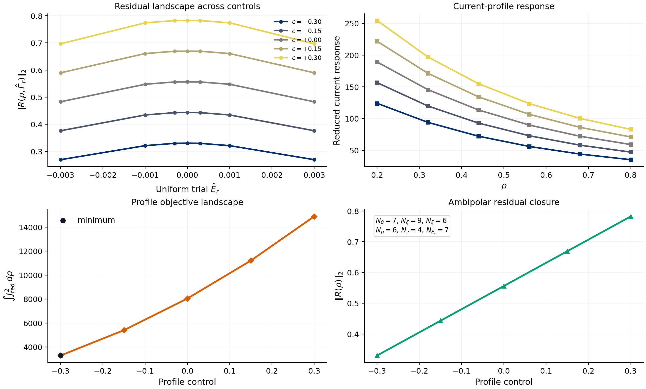
The repository example
python examples/ambipolar_profile_family.py
writes:
docs/_static/ambipolar_profile_family.png
docs/_static/ambipolar_profile_family.pdf
It shows:
the integrated residual landscape across the control family
the resulting family of reduced bootstrap-current responses
a scalar objective landscape across the control parameter
the final ambipolar residual norm across that family
Differentiable Profile-Control Optimization
On top of the family solve, NTX now exposes a scalar control optimization:
where c is a scalar profile control, w(r) is an optional radial weight, and
\lambda is a residual penalty.
The corresponding helpers are:
ProfileControlSpecapply_profile_control(...)optimize_profile_control(...)
The scalar-control implementation lives in
src/ntx/_profiles_control_scalar.py; the compatibility facade
src/ntx/_profiles_controls.py preserves the existing public import surface.
The fast test suite gates the intended linear response: zero control leaves
A1 and A3 unchanged, and finite control multiplies each species profile by
the prescribed response factor.
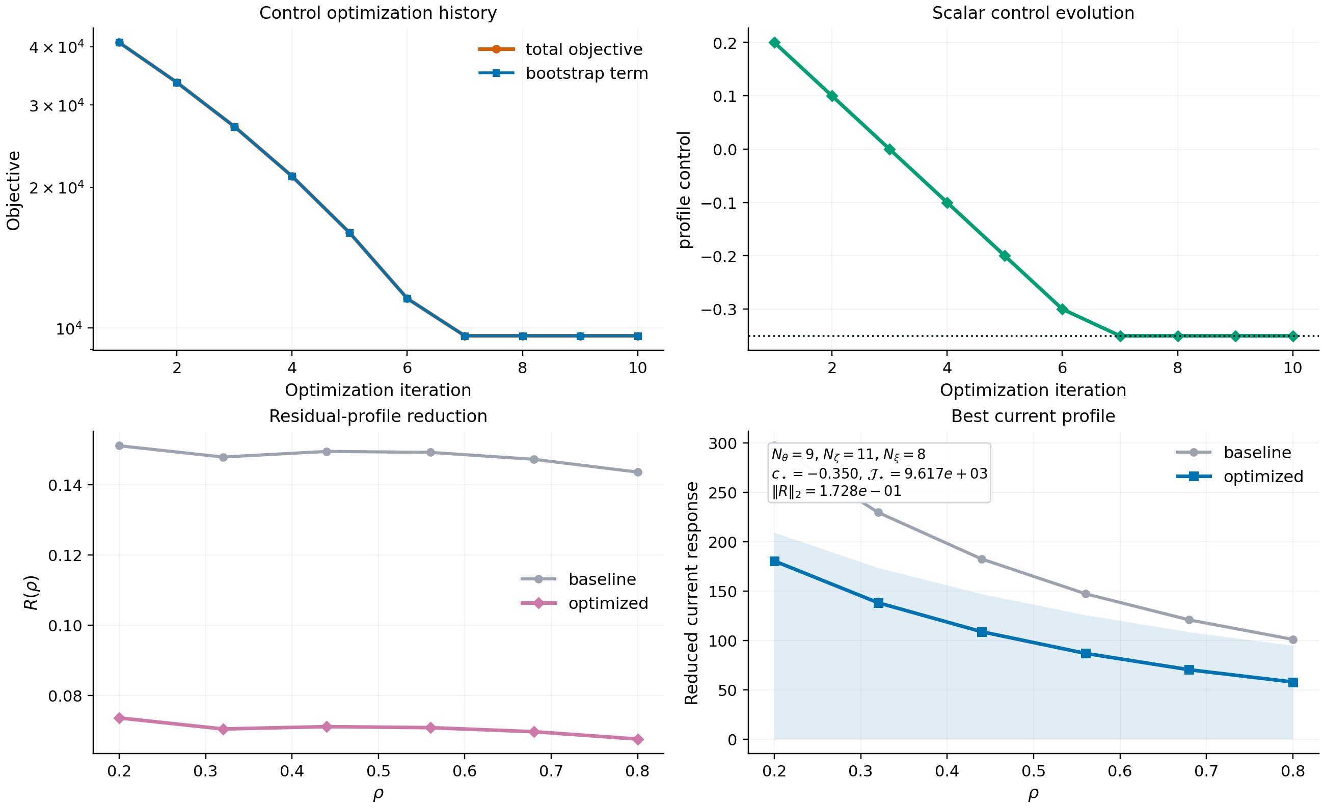
The repository example
python examples/profile_control_optimization.py
writes:
docs/_static/profile_control_optimization.png
docs/_static/profile_control_optimization.pdf
It shows:
objective descent across optimization iterations
scalar control updates
the residual-profile reduction relative to the uncontrolled baseline
the best reduced bootstrap-current response profile
The implementation lives entirely in
src/ntx/profiles.py, so the optimization stays in
the imported JAX lane instead of leaving the NTX runtime.
Low-Dimensional Radial Basis Controls
For richer profile optimization studies, NTX also exposes a low-dimensional radial basis control:
where:
c_kare the optimized basis amplitudes\phi_k(r)are user-supplied radial basis functionsR^{(1)}_{a,k}andR^{(3)}_{a,k}map each basis function into each species
The profile objective then becomes
In the current implementation, the optimization step is stabilized in two ways:
the control update uses a normalized gradient direction rather than the raw gradient magnitude
a small backtracking line search rejects steps that increase the objective
This keeps the public examples in a physically interpretable regime even when the reduced bootstrap-current response changes rapidly with control amplitude.
The corresponding helpers are:
ProfileBasisControlSpecapply_profile_basis_control(...)optimize_profile_basis_control(...)
The radial-basis implementation lives in src/ntx/_profiles_control_basis.py.
The matching gate checks that the basis-control modifier is exactly the
contracted response-basis map, with zero control again preserving the original
thermodynamic-force profiles.
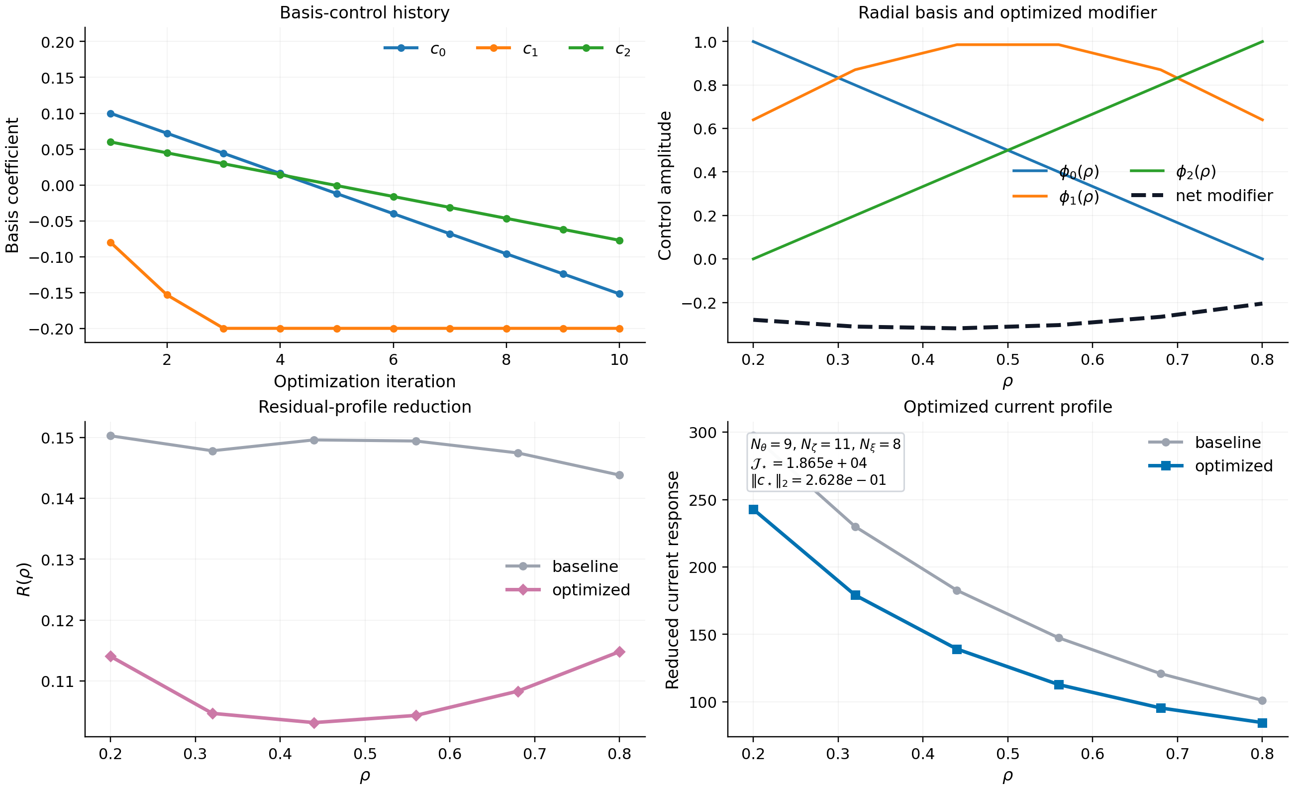
The repository example
python examples/profile_basis_optimization.py
writes:
docs/_static/profile_basis_optimization.png
docs/_static/profile_basis_optimization.pdf
docs/_static/profile_basis_optimization.json
It shows:
the basis-coefficient history
the basis functions and the final optimized modifier
the residual-profile reduction relative to the uncontrolled baseline
the optimized reduced bootstrap-current response profile
The JSON sidecar records the objective improvement, residual norm ratio, and optimized basis coefficients so this profile-basis workflow can be tracked as a stress artifact rather than only as a picture.
Profile Transport Relaxation Loop
The next step beyond explicit control families is a simple self-consistent transport-relaxation loop. NTX now exposes
ProfileTransportClosureSpecprofile_transport_loss(...)advance_profile_transport(...)solve_profile_transport_loop(...)
The closure updates the profile-force channels explicitly after each ambipolar solve, using prescribed source and target channels:
where the normalized mismatches are
The loop records a quadratic transport mismatch loss,
Each explicit update is then checked with a short backtracking acceptance rule: the next state is kept only if the recomputed transport loss does not increase. This makes the shipped workflow materially stronger than the older raw-response relaxation loop and removes the large runaway profiles that were easy to trigger in coarse public examples.
The closure-spec fields are therefore:
particle_relaxationcurrent_relaxationparticle_targetcurrent_targetparticle_sourcecurrent_sourcenormalization_floormax_normalized_updateradial_smoothing_strength
The simple default update is still explicit, but it is now much more robust for publication-facing profile studies.
The corresponding helpers are:
ProfileTransportClosureSpecprofile_transport_loss(...)advance_profile_transport(...)solve_profile_transport_loop(...)PrimitiveSpeciesProfilebuild_species_profile_from_primitives(...)build_species_profiles_from_primitives(...)primitive_profile_transport_loss(...)advance_primitive_profile_transport(...)solve_primitive_profile_transport_loop(...)
The old raw-update form,
is retained only as intuition. The shipped implementation uses the normalized source/target mismatch form above.
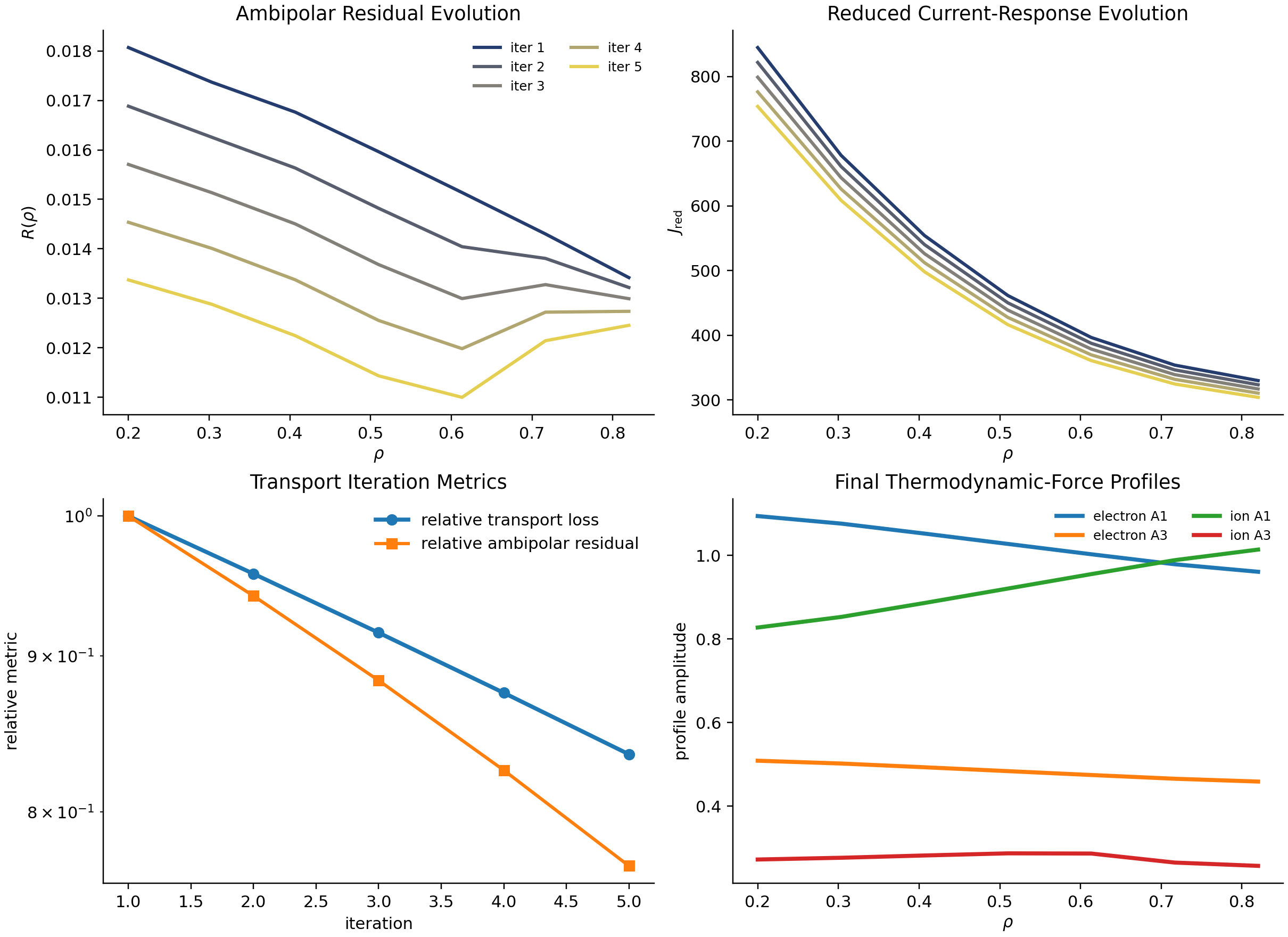
The repository example
python examples/profile_transport_loop.py
writes:
docs/_static/profile_transport_loop.png
docs/_static/profile_transport_loop.pdf
It shows:
the ambipolar residual evolution across accepted transport iterations
the corresponding reduced bootstrap-current response history
the transport-loss and ambipolar-residual histories
the final
A1(r)andA3(r)profiles for each species
Primitive Density And Temperature Transport
NTX also now supports a stronger imported workflow in which the thermodynamic forces are reconstructed from primitive density and temperature profiles rather than updated directly. For one species,
where C_{E,a}(r) is the user-supplied electrostatic prefactor. This mapping
is covered by a fast analytical physics gate and implemented by:
PrimitiveSpeciesProfilebuild_species_profile_from_primitives(...)build_species_profiles_from_primitives(...)
The primitive closure uses the same normalized transport mismatches as the
explicit A1/A3 loop, augments them with explicit density and temperature
source-target channels, and updates the primitive fields multiplicatively:
Here
with the same normalized-and-clipped structure used for the monoenergetic
transport channels. NTX then applies radial smoothing to the updated primitive
profiles before reconstructing A1(r) and A3(r) for the next ambipolar solve.
This keeps density and temperature positive, suppresses coarse-grid spikes, and
still feeds their gradients back into the ambipolar closure through A1(r) and
A3(r).
The additional primitive-closure fields on ProfileTransportClosureSpec are:
density_relaxationtemperature_relaxationdensity_targettemperature_targetdensity_sourcetemperature_sourceprimitive_normalization_floormax_primitive_normalized_updateradial_smoothing_strength
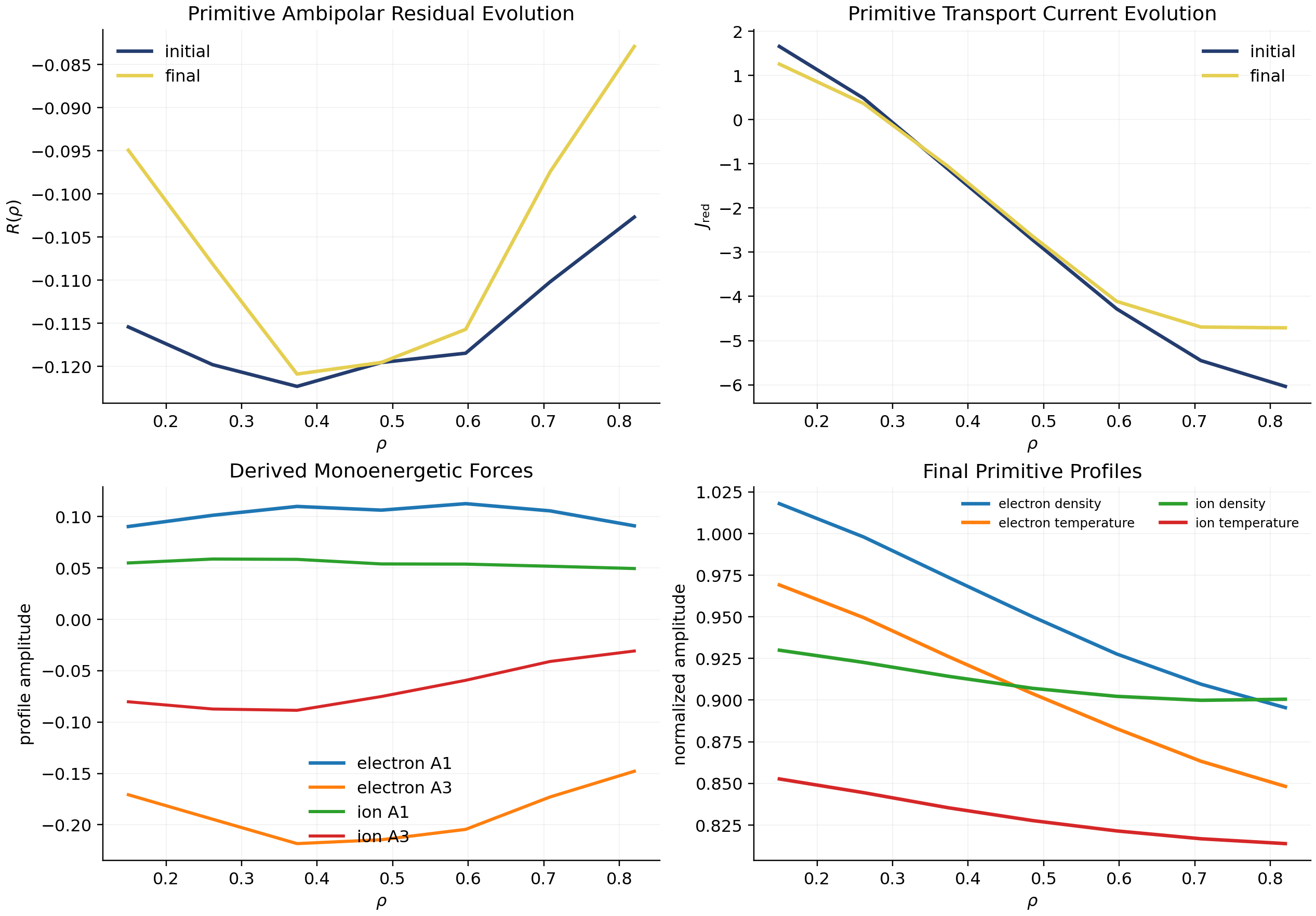
The repository example
python examples/primitive_profile_transport.py
writes:
docs/_static/primitive_profile_transport.png
docs/_static/primitive_profile_transport.pdf
and shows:
the initial-versus-final primitive ambipolar residual and current profiles
the derived monoenergetic force profiles reconstructed from the primitive state
final density and temperature profiles for each species
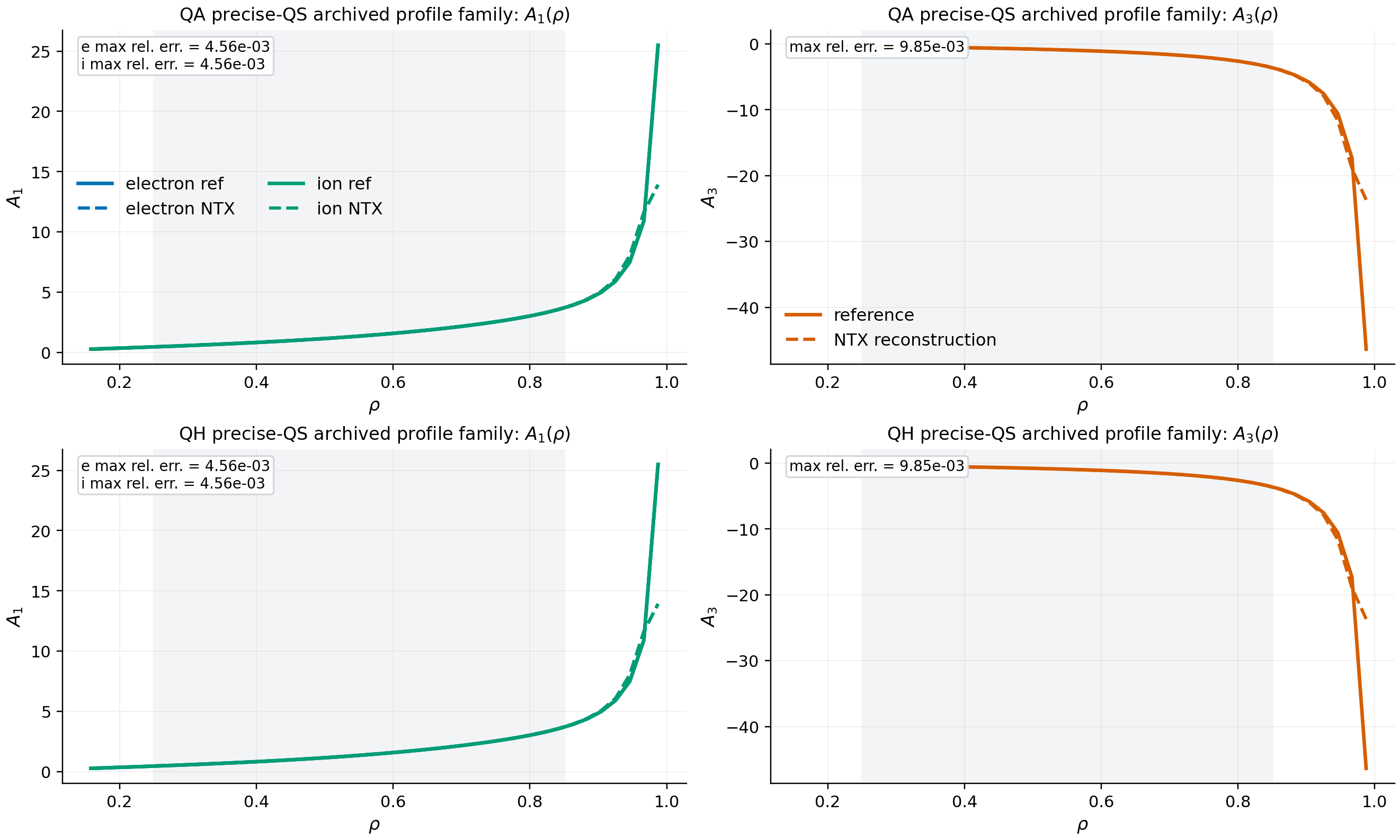
Literature-Anchored Primitive-To-Force Audit
The repository also includes a benchmark-family audit for the primitive profile reconstruction itself:
python examples/profile_force_reconstruction_audit.py
This writes:
docs/_static/profile_force_reconstruction_audit.png
docs/_static/profile_force_reconstruction_audit.pdf
docs/_static/profile_force_reconstruction_audit.json
It compares the reconstructed
profiles against the exact derivatives implied by the archived precise-QS QA/QH profile family. This is the first literature-anchored validation surface for the imported primitive-profile workflow itself, but it should be read as a coarse benchmark-family stress test for the current reconstruction scheme, not as a parity gate. It is still the right figure to carry into the paper when discussing how NTX reconstructs monoenergetic force profiles from archived benchmark inputs.
Source-Code Map
scan construction:
src/ntx/neopax.pychannel interpolation and profile closure:
src/ntx/profiles.pylow-level monoenergetic solve:
src/ntx/solver.py