NEOPAX
NTX can act as the monoenergetic coefficient provider for NEOPAX workflows.
This page describes the interfaces exposed by src/ntx/neopax.py
and when to use each of them.
Main Objects
NeopaxScan
Structured scan payload storing:
rhonu_vErEsdrdsD11D13D33
plus optional metadata and normalization arrays.
NeopaxMonoenergeticArrays
Pure-array payload designed for imported JAX workflows. This is the preferred object when the caller wants to stay in array land and avoid a hard dependency on the NEOPAX Python package.
Main Helpers
build_ntx_neopax_scan(...)build_ntx_neopax_scan_from_surfaces(...)scan_to_neopax_arrays(...)to_neopax_monoenergetic(...)write_neopax_scan_hdf5(...)load_neopax_reference_scan(...)build_differentiable_neopax_field_from_vmec_booz_files(...)
The imported profile layer in src/ntx/profiles.py
builds directly on NeopaxScan when the next step is an ambipolar or
reduced bootstrap-current response solve instead of immediate export into the
external package object.
For end-to-end examples, see:
examples/neopax_with_ntx.pyfor the smallest scan-to-array workflowexamples/owned_geometry_neopax_dataset.pyfor an owned finite-betavmex -> booz_xform_jax -> NTX -> NEOPAXdataset, direct wout-harmonic stress cases, and interpolation-path auditexamples/owned_finite_beta_sfincs_jax_inputs.pyfor same-grid SFINCS-JAX input generation, completed-output ingestion, and coefficient-level NTX comparison before any finite-betaSFINCS/Redl/NTX+NEOPAXparity promotionexamples/owned_finite_beta_sfincs_jax_resolution_audit.pyfor the production stress-radius coefficient-resolution and harmonic-cutoff audit that keeps the finite-beta current gap out of hidden numerical knobsexamples/owned_finite_beta_sfincs_jax_production_ladder_audit.pyfor the production radius/collisionality coefficient ladder that localizes the remaining finite-beta stress to the profile-current closure layerexamples/owned_finite_beta_sfincs_jax_profile_current_audit.pyfor the direct RHSMode=1 profile-current diagnostic on the same finite-beta VMEC/profile contract used by Redl andNTX+NEOPAXexamples/owned_finite_beta_sfincs_jax_profile_current_resolution_audit.pyfor the pitch Legendre truncation audit that closes the finite-beta reduced-closure stress lane at the documented high-Nxitoleranceexamples/owned_finite_beta_bootstrap_comparison.pyfor an owned finite-beta Redl andNTX+NEOPAXbootstrap-current stress audit on the same VMEC wout, Boozer transform, profiles, radial grid, and current normalizationexamples/owned_finite_beta_closure_localization.pyfor the sidecar that separates same-grid coefficient error from the remaining finite-beta profile-current closure gapexamples/owned_finite_beta_profile_current_observable_audit.pyfor the finite-beta stress-radius observable decomposition into no-momentum current, momentum correction, correction needed to match Redl, species-current cancellation scale, and Pmax trendexamples/owned_finite_beta_current_conditioning_audit.pyfor the cancellation-conditioned coefficient-precision requirement that must be met before the finite-beta net-current residual is assigned to a reduced closure changeexamples/owned_finite_beta_closure_quadrature_audit.pyfor the Sonine-order versus velocity-quadrature audit that rejects under-integrated apparent finite-beta current-gate passesexamples/owned_finite_beta_source_channel_audit.pyfor the stress-radius physical source-channel decomposition of the same momentum-restoring linear systemexamples/owned_finite_beta_source_response_profile_audit.pyfor the profile-wide effective-temperature source-response map against Redl collisionality and geometry driversexamples/owned_finite_beta_closure_target_audit.pyfor the closure-target driver ranking that turns the profile source-response map into a runtime-neutral design diagnosticexamples/bootstrap_current_with_neopax.pyfor a radial bootstrap-current profile built from an NTX scan and evaluated through NEOPAXexamples/bootstrap_current_fixed_field_validation.pyfor the local precise-QS fixed-field comparison against SFINCS, SFINCS-JAX, and Redlexamples/build_neopax_scan_from_ertilde.pyfor generating a NEOPAX-style HDF5 coefficient database directly from VMEC/Boozer files and a user-providedrho,nu_v, andEr_tildegridexamples/boozmn_backend_validation_audit.pyfor dumping the direct Boozer-file geometry, radial-drift source, operator channels, and transport coefficients against the validated VMEC-harmonic pathexamples/boozmn_same_coordinate_roundtrip_audit.pyfor the same-coordinate VMEC half-grid Boozer-file round-trip gate that validates directboozmnloading before representation-comparison claims
Typical Imported Workflow
import jax.numpy as jnp
from ntx import (
    GridSpec,
    build_ntx_neopax_scan,
    scan_to_neopax_arrays,
    surface_from_vmex_vmec_wout_file,
)

rho = jnp.linspace(0.2, 0.8, 5)
nu_v = jnp.logspace(-5, -2, 8)
Es = jnp.zeros((rho.size, 6))
Er = jnp.zeros_like(Es)
drds = jnp.ones_like(rho)

def surface_loader(rho_value: float):
    return surface_from_vmex_vmec_wout_file("wout.nc", s=float(rho_value**2))

scan = build_ntx_neopax_scan(
    surface_loader,
    rho=rho,
    nu_v=nu_v,
    Es=Es,
    Er=Er,
    drds=drds,
    grid=GridSpec(n_theta=17, n_zeta=25, n_xi=32),
)

arrays = scan_to_neopax_arrays(scan, a_b=1.0)
By default, the conversion keeps the raw D33 database convention used by the
integrated workflow:
arrays = scan_to_neopax_arrays(scan, a_b=1.0, d33_mode="raw")
The d33_mode="spitzer" and d33_mode="conductivity_difference" branches are
explicit audit choices. They are useful for fixed-field closure stress tests,
but they are not the public default because they do not satisfy the integrated
W7-X transfer gate.
DKES-Like Er_tilde Database Export
When the downstream workflow expects a file-backed coefficient database, use
the Er_tilde export example instead of hand-editing HDF5 payloads:
python examples/build_neopax_scan_from_ertilde.py \
  --wout path/to/wout.nc \
  --booz path/to/boozmn.nc \
  --rho 0.25,0.5,0.75 \
  --nu-v 1e-5,3e-5,1e-4,3e-4,1e-3 \
  --er-tilde 0.0,1e-5,3e-5 \
  --surface-backend vmec \
  --device-backend cpu \
  --scan-batch-size 32 \
  --output examples/outputs/neopax_scan_from_ertilde/scan.h5 \
  --plot
The script validates the input files and grids, computes Er, Es, and
normalization metadata from the supplied VMEC/Boozer files, solves the NTX
monoenergetic coefficient tables, writes write_neopax_scan_hdf5(...) output,
and can emit per-radius coefficient panels for quick sanity checks.
Use the VMEC surface backend for validation and benchmark generation. The
boozmn backend is available as an explicit geometry-backend audit path, but
it is not the default validation path.
--scan-batch-size bounds memory inside each radial-surface scan. It is not
itself a CPU parallelism switch. For CPU-only laptops, expose multiple JAX host
devices before Python imports JAX, then request sharding explicitly:
XLA_FLAGS=--xla_force_host_platform_device_count=4 \
python examples/build_neopax_scan_from_ertilde.py \
  --wout path/to/wout.nc \
  --booz path/to/boozmn.nc \
  --surface-backend vmec \
  --device-backend cpu \
  --parallel-devices 4 \
  --scan-batch-size 32 \
  --output examples/outputs/neopax_scan_from_ertilde/scan.h5
If --device-backend gpu is requested on a CPU-only laptop, the script now
fails with the available JAX platforms and tells the user to switch to
--device-backend cpu. Also check
python examples/build_neopax_scan_from_ertilde.py --help: if
--scan-batch-size and --parallel-devices are missing, the local NTX checkout
or installed package is stale.
For the QI finite-beta hires example used in downstream database generation,
the full-surface vectorized scan is GPU-friendly but memory-heavy on CPU. On
the local CPU reference run, 25 x 25 x 60 with one radial surface and the
default 16 x 12 (nu_v, Er_tilde) grid took 64.7 s and about 5.0 GB
peak RSS. Adding --scan-batch-size 32 reduced that to 55.9 s and about
1.46 GB peak RSS for the same coefficients. Smaller batches such as 16
lower memory further but were slower in this probe, so 32 is the recommended
CPU fallback for this case. Leave the option unset on GPU unless device memory
is the limiting factor.
Direct Boozer-File Backend Audit
boozmn spectra and Boozer radial profiles are half-grid quantities. The
direct loader therefore selects and interpolates packed B_{mn} surfaces using
s_in, s_b, or jlist = compute_surfs + 2, not the full-grid toroidal-flux
profile phi_b. The same-coordinate round-trip gate is the first check:
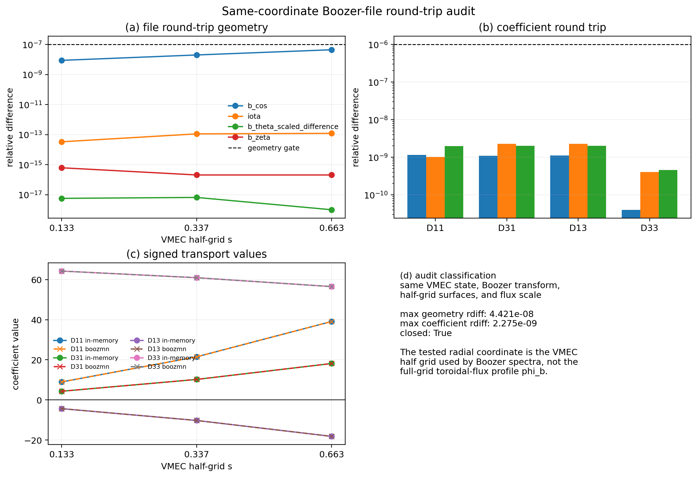
python examples/boozmn_same_coordinate_roundtrip_audit.py
This script generates a Boozer file from a VMEC wout, reloads the same
half-grid surfaces through load_boozmn_surface(...), and compares geometry
metadata plus D11/D31/D13/D33 with the in-memory
vmex -> booz_xform_jax -> NTX path. A passing gate validates the direct
file loader. It does not imply that a VMEC-harmonic representation and a
direct Boozer-coordinate representation have identical source channels.
The direct Boozer-file path and the VMEC-harmonic path do not expose identical
coordinate channels. The direct Boozer helper represents the magnetic field in
Boozer coordinates with flux-function covariant components, while the
VMEC-harmonic helper reads the signed VMEC Jacobian and angle-dependent
covariant/contravariant channels from the wout file. Because the NTX
monoenergetic source contains
backend promotion must be based on this source channel, not only on close
B_{00} or D_{33} values.
Run the backend audit before using direct boozmn surfaces for benchmark
claims:
python examples/boozmn_backend_validation_audit.py \
  --wout path/to/wout.nc \
  --boozmn path/to/boozmn.nc \
  --rho 0.5 \
  --nu-hat 1e-2 \
  --epsi-hat 0.0
The audit writes JSON plus PNG/PDF panels with the surface metadata, geometry
statistics, s1/s3 source norms, k=1 operator-channel norms, signed
D11/D31/D13/D33 values, and relative differences against the VMEC-harmonic
path. Direct Boozer-file output should stay in audit mode unless both the
transport-coefficient and radial-drift source differences pass on owned
same-coordinate cases. A failing audit localizes a convention or interpolation
gap; it is not a reason to introduce fitted closure constants.
When converting NEOPAX parallel-flow output into current, use one charge
conversion only. If the workflow uses species.charge, that array already
contains the signed physical charge in Coulombs. If the workflow uses
species.charge_qp, multiply by one elementary-charge factor:
current = elementary_charge * np.sum(species.charge_qp[:, None] * upar, axis=0)
JAX-Native Geometry Workflows
Use the matching VMEC input and wout when the geometry should stay inside the
JAX geometry stack and the Boozer transform should be owned by the same run:
import jax.numpy as jnp
from ntx import GridSpec, build_ntx_neopax_scan_from_surfaces, surface_from_vmex_wout

rho = jnp.asarray([0.35, 0.65])
psi_p = 0.013346299916410087  # abs(phi_edge)/(2*pi) from the matching wout
surfaces = tuple(
    surface_from_vmex_wout(
        input_path="input.LandremanPaul2021_QA_lowres_pressure_current",
        wout_path="wout_LandremanPaul2021_QA_lowres_pressure_current.nc",
        s=float(rho_value**2),
        mboz=4,
        nboz=4,
        psi_p=psi_p,
    )
    for rho_value in rho
)

scan = build_ntx_neopax_scan_from_surfaces(
    surfaces,
    rho=rho,
    nu_v=jnp.asarray([1.0e-3, 1.0e-2]),
    Es=jnp.zeros((rho.size, 1)),
    drds=jnp.ones_like(rho),
    grid=GridSpec(7, 7, 6),
    source_name="owned-finite-beta-qa",
)
surface_from_vmex_vmec_wout_file(...) is still useful when only a wout
file is available. It reads the VMEC harmonic tables through vmex and
uses NTX’s radial interpolation of those tables. That path is not identical to
the Boozer-transform path above, so the two should be compared only as an
interpolation/geometry-loader audit on the same owned input family.
For physical-current or NEOPAX database workflows, do not rely on the
low-level Boozer helper’s default psi_p=1. Pass the VMEC edge toroidal flux
divided by 2*pi explicitly. The owned finite-beta diagnostic records this
value in its JSON sidecar and uses it to keep the Boozer-coordinate and direct
VMEC-harmonic transport paths on the same flux normalization.
When building a NEOPAX-style field object from VMEC and boozmn files, use
build_differentiable_neopax_field_from_vmec_booz_files(...). Boozer B00
profiles are tabulated on normalized radius, so the helper evaluates B00 on
rho and converts the derivative with dB00/dr = (dB00/d rho)/a_b. This is the
normalization used by the finite-beta bootstrap-current stress artifacts.
For in-memory differentiable studies, avoid file-backed geometry loops and use
build_ntx_neopax_scan_from_vmex_state(...) or
build_ntx_neopax_scan_from_vmex_boundary_params(...). Those helpers keep
the VMEC state, Boozer transform, NTX scan, and NEOPAX-style arrays on the
JAX-facing path used by the derivative examples.
Explicit-Surface Workflow
If the surfaces are already in memory, avoid the callback boundary:
from ntx import build_ntx_neopax_scan_from_surfaces

scan = build_ntx_neopax_scan_from_surfaces(
    surfaces,
    rho=rho,
    nu_v=nu_v,
    Es=Es,
    Er=Er,
    drds=drds,
    grid=grid,
)
This is the cleaner choice for JAX-native surface-generation pipelines.
HDF5 Workflow
Load a NEOPAX-style monoenergetic table:
from ntx import load_neopax_reference_scan

scan = load_neopax_reference_scan("monoenergetic.h5")
Write one:
from ntx import write_neopax_scan_hdf5

write_neopax_scan_hdf5(scan, "monoenergetic_out.h5")
The writer stores uncompressed numeric datasets with HDF5 object timestamps disabled. That keeps repeated database regeneration fast and avoids needless binary churn from file metadata.
Conversion Layers
JAX-friendly path
scan_to_neopax_arrays(...)
Use this when:
the next step is still JAX-based
gradients matter
the caller wants direct access to the normalized arrays
Convenience object path
to_neopax_monoenergetic(...)
Use this when the NEOPAX package is installed and the goal is to hand the data to NEOPAX directly as a Python object.
What NTX Supplies To NEOPAX
NTX supplies the monoenergetic geometric coefficients on the requested radial, collisionality, and electric-field grid. NEOPAX then uses those tables in its own higher-level transport workflow.
That separation of responsibility is deliberate:
NTX owns the monoenergetic solve
NEOPAX owns the radial multi-species transport layer
Profile-Grade Imported Workflows
When the next step is still inside NTX, use the profile helpers on top of the scan payload:
evaluate_scan_channel(...)evaluate_species_particle_flux(...)evaluate_species_current_response(...)ambipolar_residual_profile(...)solve_ambipolar_er_profile(...)solve_ambipolar_profile_family(...)bootstrap_current_objective(...)apply_profile_control(...)optimize_profile_control(...)apply_profile_basis_control(...)optimize_profile_basis_control(...)advance_profile_transport(...)profile_transport_loss(...)solve_profile_transport_loop(...)
Those helpers are documented on the Profiles page.