Geometry And Inputs
NTX can solve the monoenergetic problem from four geometry families:
the built-in analytic sample surface
DKES-style Boozer harmonic files
VMEC
woutfiles throughvmexBoozer
boozmnfiles throughbooz_xform_jax
This page explains how those inputs are turned into the common internal representation used by the solver.
Internal Surface Objects
NTX has two main surface dataclasses in
src/ntx/geometry.py:
BoozerSurfaceVmecSurface
Both are JAX pytrees, so they can be passed through jit, vmap, and grad
in the imported lane.
Boozer Harmonic Surfaces
BoozerSurface stores:
integer mode arrays
m,nFourier coefficients
b_cosand optionalb_sinfield-period count
nfprotational transform
iotaflux normalization
psi_pcovariant Boozer field components
B_theta,B_zetaoptional
B0
The Fourier evaluator in
src/ntx/geometry.py computes
and returns B, \partial_\theta B, and \partial_\zeta B directly from the
trigonometric series.
DKES-Style Files
load_dkes_surface(...) in src/ntx/io.py parses
ddkes2.data-style inputs and fills BoozerSurface.
Use this path when:
a Boozer harmonic surface is already available
the goal is a direct monoenergetic solve without VMEC preprocessing
VMEC wout Files
load_vmec_surface(...) in src/ntx/vmec.py reads
VMEC equilibria through vmex and extracts a single surface.
The loader resolves:
nfp,ns,mpol,ntoriota(\psi_n)Fourier coefficients for:
BJacobian
B_\theta,B_\zetaB^\theta,B^\zeta
psi_a_hatAminor_pthe electric-field transport normalization
VMEC Knobs
The VMEC loader exposes four important knobs.
psi_n
The requested normalized toroidal-flux label.
vmec_radial_option
0: interpolate to the requestedpsi_n1: snap to the nearest interior VMEC surface2: snap to the nearest VMEC surface including endpoints
This affects whether NTX uses the exact requested radial location or a discrete surface from the VMEC radial grid.
vmec_nyquist_option
1: reduced mode set2: keep Nyquist modes
vmec_mode_convention
"reduced": use the reduced VMEC(xm, xn)table"filtered_nyquist": retain the Nyquist subset satisfying the mode filters
min_bmn_to_load
Discard modes whose relative amplitude |B_mn/B_00| is below the threshold.
This is a practical performance control. It reduces harmonic count, memory traffic, and transform cost when very small modes are not needed.
Boozer boozmn Files
NTX can also load Boozer harmonic files directly through the Python/JAX Boozer
helpers in src/ntx/booz.py.
Use this path when:
the equilibrium has already been transformed to Boozer coordinates
the workflow is based on Boozer harmonics instead of VMEC harmonics
In that case, NTX bypasses VMEC interpolation and goes directly to
BoozerSurface.
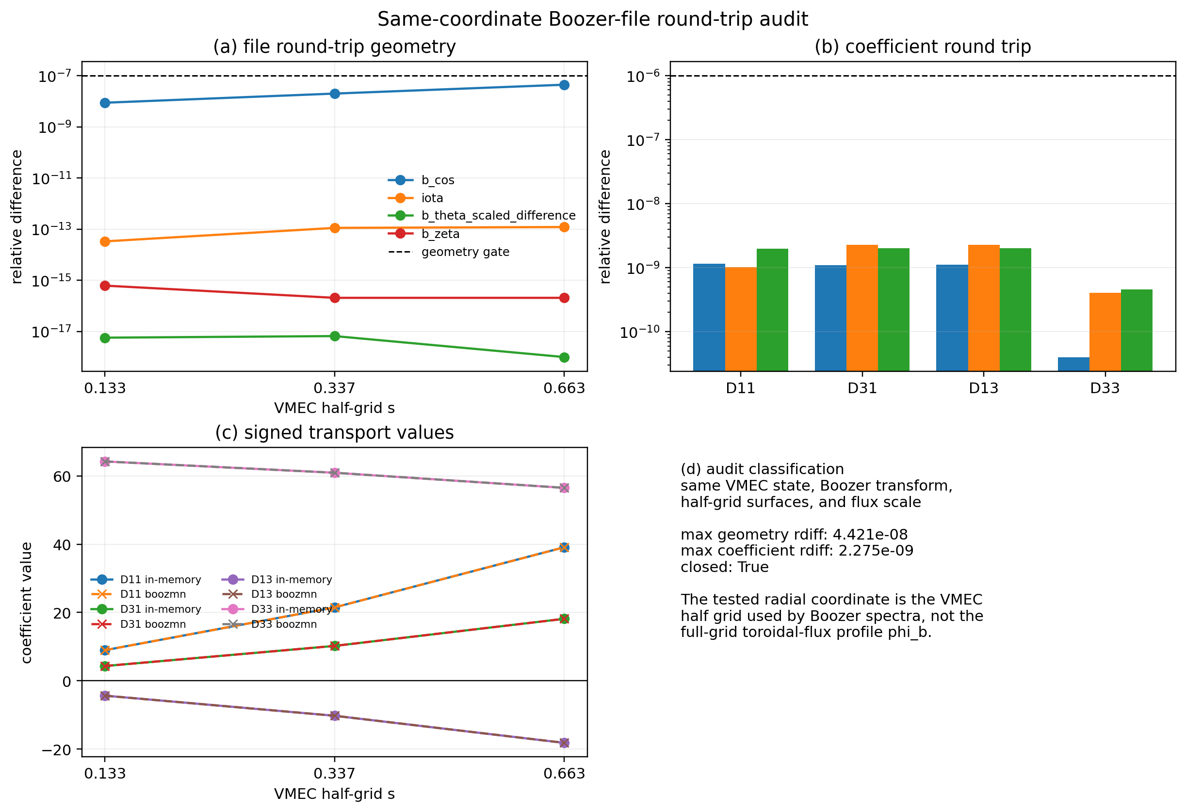
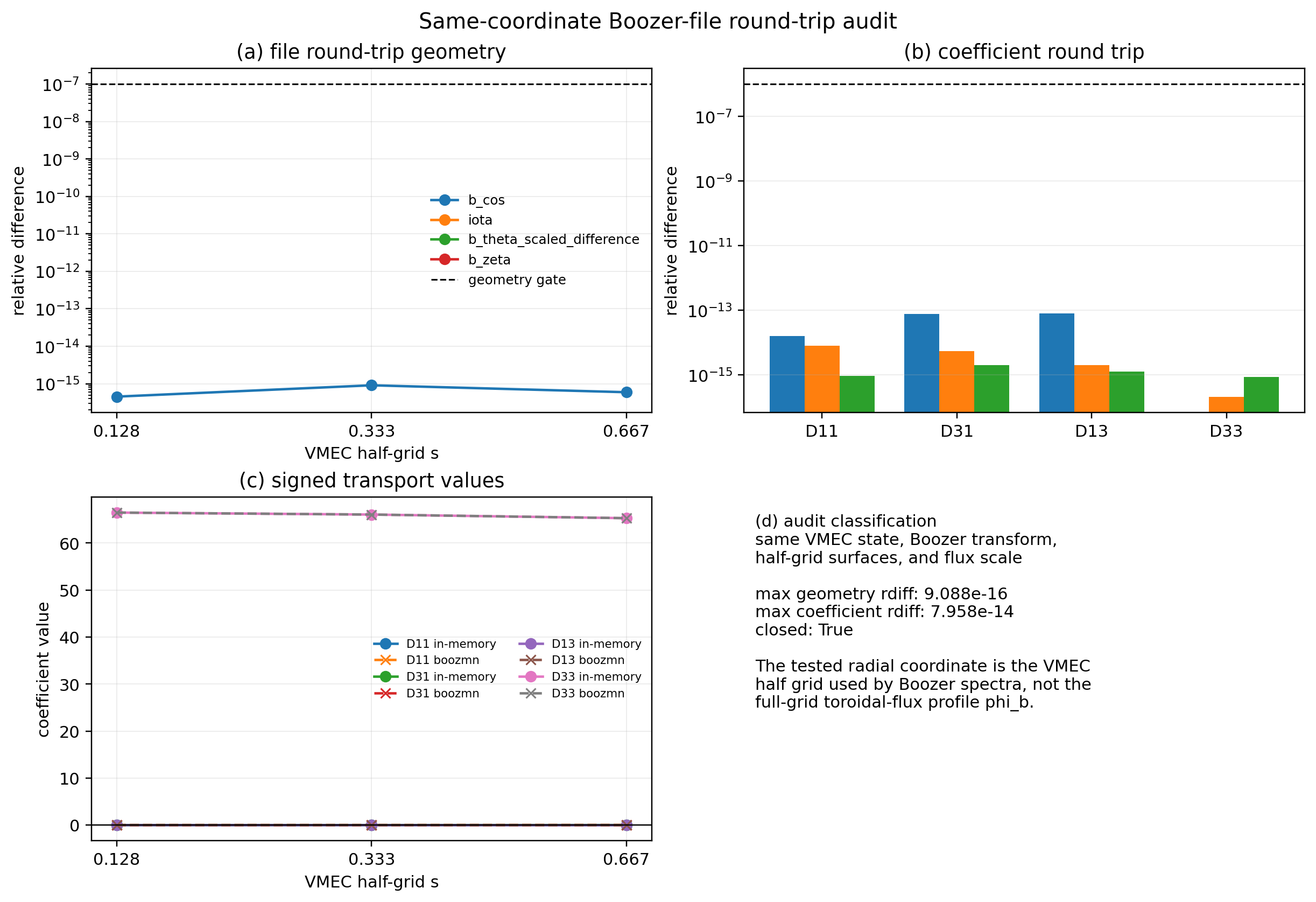
The direct boozmn loader treats Boozer spectra and Boozer radial profiles as
VMEC half-grid quantities. In modern boozmn files this information is exposed
through s_in, s_b, and the packed-surface jlist convention, where
jlist = compute_surfs + 2. The full-grid toroidal-flux profile phi_b is
metadata and is not the radial coordinate for selecting packed B_{mn}
surfaces. This matters because a full-grid shift changes the selected surface
and therefore the magnetic-drift source before any closure or current-profile
normalization is reached.
The maintained same-coordinate round-trip audit is:
python examples/boozmn_same_coordinate_roundtrip_audit.py
It generates a boozmn file from a VMEC wout, reloads the same VMEC
half-grid surfaces through load_boozmn_surface(...), and compares the loaded
geometry and D11/D31/D13/D33 against the in-memory
vmex -> booz_xform_jax -> NTX path. That audit validates the direct
loader on the same coordinate representation. It is separate from audits that
compare VMEC-harmonic and Boozer-coordinate representations, since those expose
different geometry channels.
For file-backed work, surface_from_vmex_wout(..., profile_source="auto")
and profile_source="wout" use the finalized WOUT magnetic channels directly.
Current vmex intentionally removed the legacy state_from_wout
reconstruction API: a WOUT is an output representation, not a complete
differentiable equilibrium state. In-memory differentiable work instead passes
the converged SpectralState and matching SolverRuntime to
surface_from_vmex_state(...); NTX then uses the traceable
vmex.core.boozer_tables.boozer_input_tables bridge. Neither path applies
a fitted correction.
The finite-beta transfer artifact exercises this path on an optimized QA
finite-beta wout and closes the same-coordinate transport mismatch to
roundoff.
Geometry Evaluation On The Angular Grid
All surface families are converted to GeometryOnGrid by
geometry_on_grid(...) in src/ntx/geometry.py.
That object stores:
theta_2d,zeta_2dB\partial_\theta B,\partial_\zeta B\mathcal JB_\theta,B_\zetaB^\theta,B^\zeta\langle B^2 \rangleV'the radial-drift source factor
the normalization scales used later by the transport coefficients
This is the canonical internal geometry representation for the solver.
Angular Domain
NTX discretizes one field period:
This is implemented in periodic_grid(...) in
src/ntx/grids.py.
Coordinate Flattening Convention
Flux-surface fields are flattened with theta as the fastest index:
flatten_fs(...)unflatten_fs(...)
in src/ntx/grids.py.
This matters for:
dense operator assembly
mode-vector interpretation
file-backed output arrays
Geometry In The CLI Output
The ntx input.toml workflow writes the evaluated geometry into the output
NetCDF, NPZ, or HDF5 file:
theta_gridzeta_gridbd_b_dthetad_b_dzetajacobianb_sub_thetab_sub_zetab_sup_thetab_sup_zetaradial_drift_spatialvolume_primeb2_mean
These are written in save_run_output(...) in
src/ntx/_inputfiles_output.py.
Recommended Input Strategy
Use
example_surface()for fast development and testing.Use DKES-style or Boozer inputs when the Boozer harmonics are already available and fixed.
Use VMEC inputs when the workflow begins from equilibrium data and radial interpolation matters.
Use the imported
vmexlane when NTX needs to sit inside a larger JAX analysis or optimization loop.