Examples
This page lists the main ways to run NTX, from the smallest CLI solve to the publication-figure scripts.
1. Simplest CLI Run
ntx examples/example_surface.toml --plot
This is the smallest end-to-end solve. It requires no external files and is the
best first command to confirm that NTX is installed correctly. It writes a
NetCDF payload and a PDF summary panel under examples/outputs/.
2. DKES-Style CLI Run
ntx examples/sample_dkes.toml
This writes a NetCDF result under examples/outputs/. Use
--output examples/outputs/sample_dkes.npz when a compact NumPy archive is
preferred.
3. VMEC CLI Run
ntx examples/sample_vmec.toml
This exercises the VMEC normalization path on the bundled sample wout file.
4. Open And Plot An Output File
python examples/plot_output_file.py examples/outputs/sample_dkes.nc
This reads an NTX .nc, .npz, or .h5 payload and writes:
docs/_static/output_file_summary.pngdocs/_static/output_file_summary.pdf
The output figure contains:
magnetic-field strength on the angular grid
the radial-drift source on the same grid
the solved transport coefficients
a run-summary panel with key diagnostics
5. Python Single-Case Solve
from ntx import GridSpec, MonoenergeticCase, load_vmec_surface, solve_monoenergetic

surface = load_vmec_surface("wout.nc", psi_n=0.25)
grid = GridSpec(n_theta=9, n_zeta=11, n_xi=12)
case = MonoenergeticCase(nu_hat=1e-3, er_hat=1e-3)
result = solve_monoenergetic(surface, grid, case)
Reusable Prepared Scans
For repeated fixed-geometry monoenergetic scans, use
compile_prepared_scan_solver(...) as shown in the README. The prepared object
keeps one fixed batch shape and exposes warmup() timing and memory metadata.
Generate a CPU/GPU crossover figure with:
python examples/prepared_scan_performance.py \
  --cpu-json docs/_static/prepared_scan_cpu_production.json \
  --gpu-json docs/_static/prepared_scan_gpu_production.json \
  --output-prefix docs/_static/prepared_scan_performance
6. NEOPAX Mapping
python examples/neopax_with_ntx.py
This example:
loads a VMEC equilibrium
builds an NTX monoenergetic scan
maps that scan into NEOPAX-style arrays
Use it as the minimal reference for NTX-to-NEOPAX coupling.
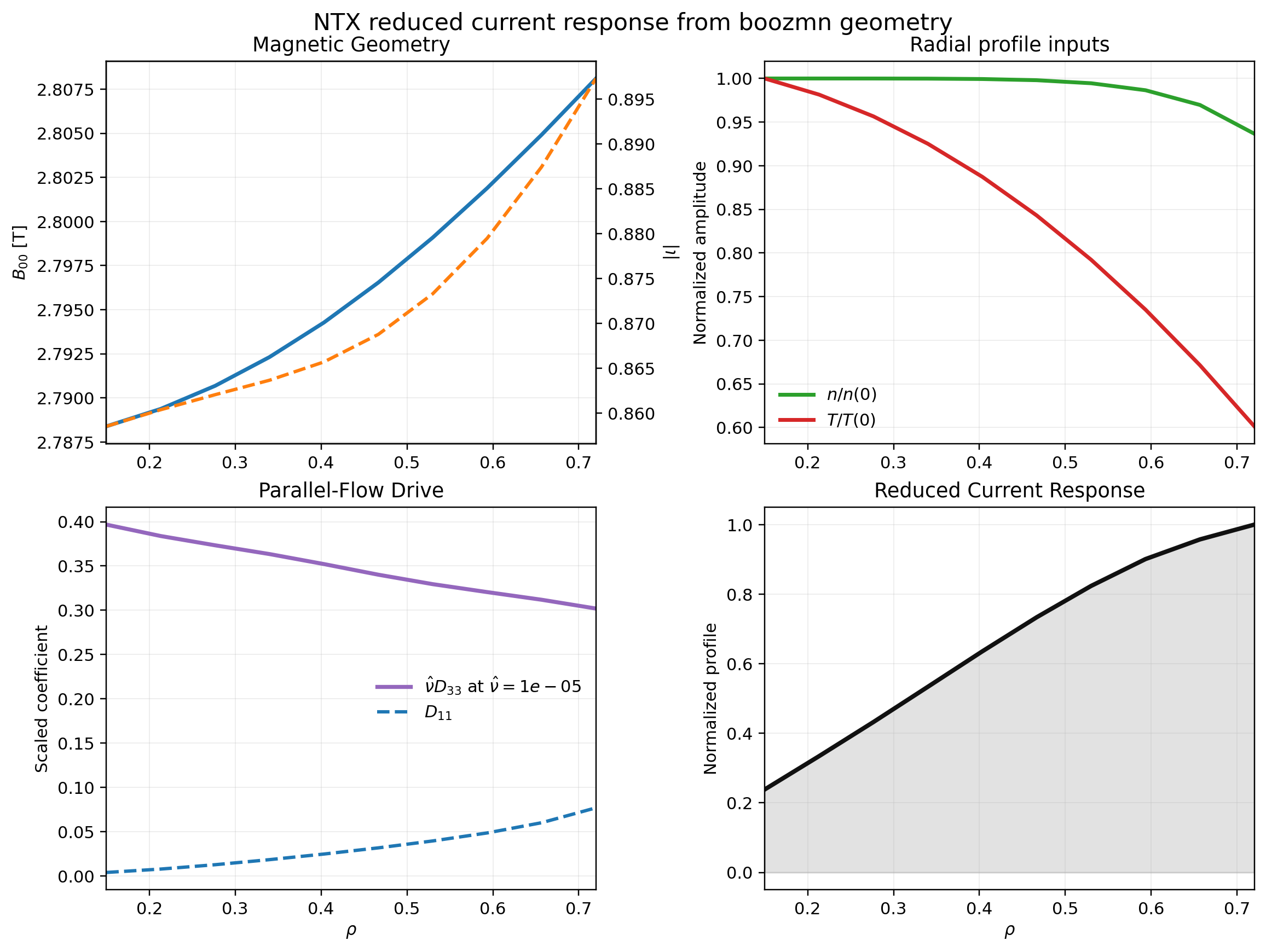
7. Bootstrap Current From VMEC Or Boozmn
python examples/bootstrap_current_from_vmec_or_boozmn.py
This example is the shortest NTX-only workflow:
start from a VMEC
woutfile and usevmexor, if a Boozer
boozmnfile already exists, usebooz_xform_jaxoutput directlysolve a fixed-collisionality NTX radial family
plot magnetic geometry, radial profile inputs,
D11,nu_hat * D33, and a compact interior reduced bootstrap-current response
All user inputs live at the top of the file. The script prefers direct Boozer
input in auto mode when a boozmn file is available and otherwise falls back
to the VMEC-harmonic lane. The density and temperature derivatives are taken
analytically in the example so the figure reflects the transport response rather
than finite-difference edge noise.
It writes:
docs/_static/bootstrap_current_from_vmec_or_boozmn.pngdocs/_static/bootstrap_current_from_vmec_or_boozmn.pdfdocs/_static/bootstrap_current_from_vmec_or_boozmn.json
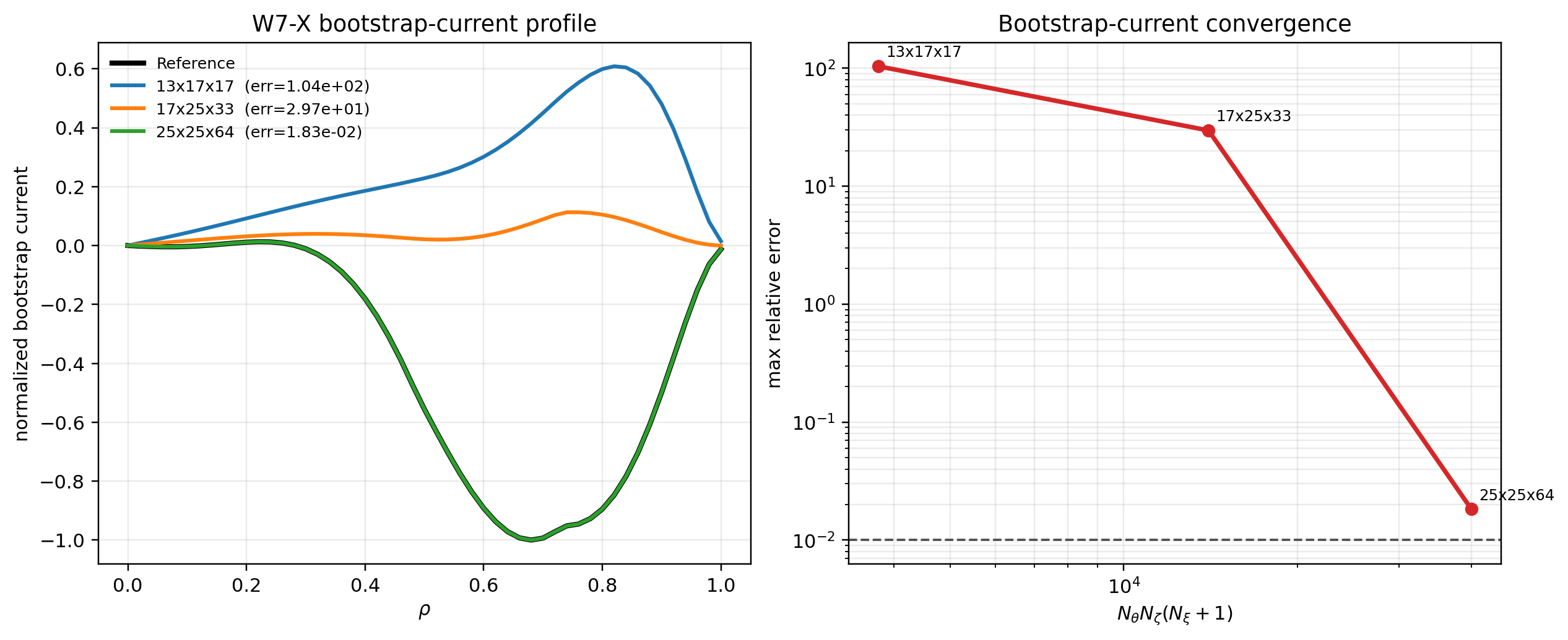
8. W7-X Bootstrap-Current Convergence Audit
python examples/bootstrap_current_reference_audit_w7x.py
This optional audit script rebuilds a reduced W7-X scan at several NTX resolutions, evaluates the resulting bootstrap-current profile through the imported workflow, and writes a convergence figure:
docs/_static/bootstrap_current_reference_audit_w7x.pngdocs/_static/bootstrap_current_reference_audit_w7x.pdfdocs/_static/bootstrap_current_reference_audit_w7x.json
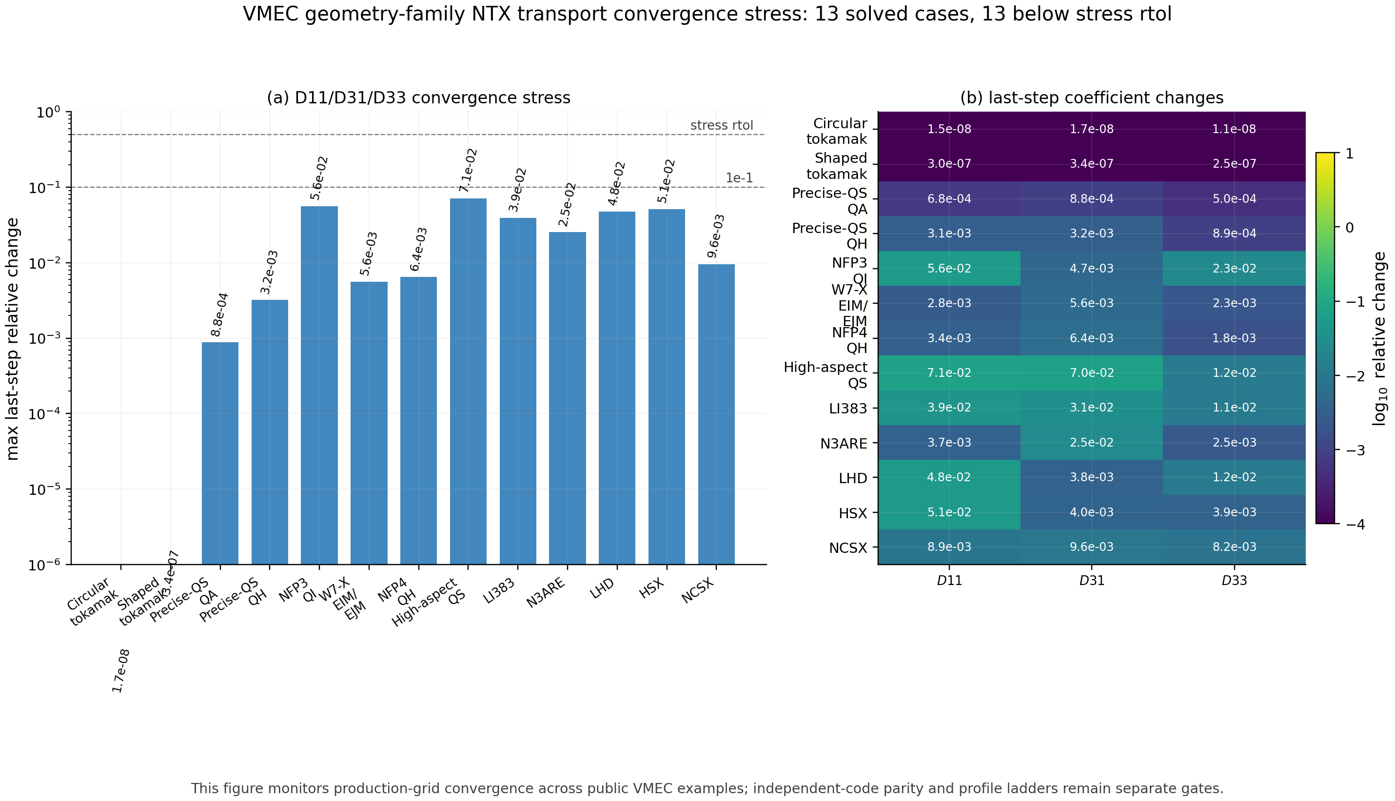
9. VMEC Geometry-Family Transport Convergence
python examples/geometry_family_transport_convergence.py --preset production
This optional artifact discovers local public VMEC examples from vmex,
STELLOPT, and SIMSOPT checkouts, then runs a production D11/D31/D33
convergence ladder and stores D13 for the Onsager quality check. It is an NTX
stress diagnostic across available geometry families, not an independent-code
parity claim.
It writes:
docs/_static/geometry_family_transport_convergence.pngdocs/_static/geometry_family_transport_convergence.pdfdocs/_static/geometry_family_transport_convergence.json
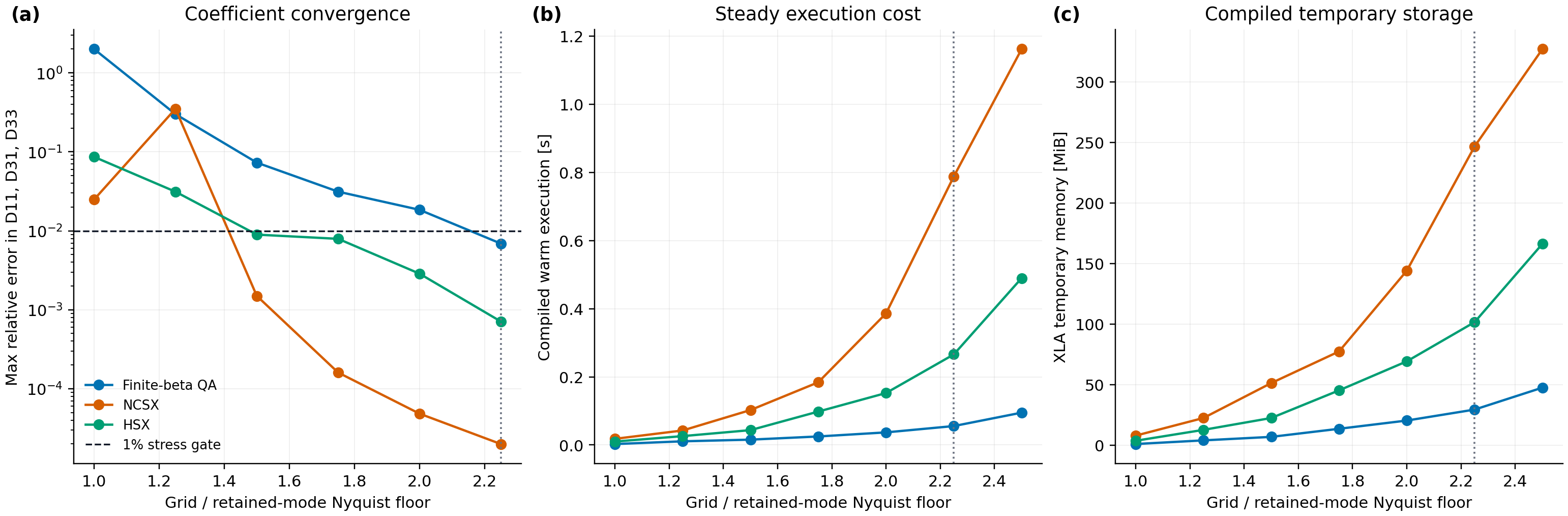
10. Angular Collocation Oversampling Audit
python examples/angular_oversampling_audit.py --preset production
This artifact uses public finite-beta QA, NCSX, and HSX VMEC equilibria to
measure D11/D31/D33 error against a finer angular grid while separately
reporting compiled warm runtime and XLA temporary memory. The measured 2.25
times Nyquist recommendation is a warning-level starting point; publication
calculations still require two successive accepted refinements.
It writes:
docs/_static/angular_oversampling_audit.pngdocs/_static/angular_oversampling_audit.pdfdocs/_static/angular_oversampling_audit.json
11. Owned JAX-Native NTX+NEOPAX Dataset
python examples/owned_geometry_neopax_dataset.py
python examples/owned_finite_beta_sfincs_jax_inputs.py
python examples/owned_finite_beta_sfincs_jax_resolution_audit.py
python examples/owned_finite_beta_sfincs_jax_production_ladder_audit.py
python examples/owned_finite_beta_sfincs_jax_profile_current_audit.py
python examples/owned_finite_beta_sfincs_jax_profile_current_resolution_audit.py
python examples/owned_finite_beta_bootstrap_comparison.py
python examples/owned_finite_beta_closure_localization.py
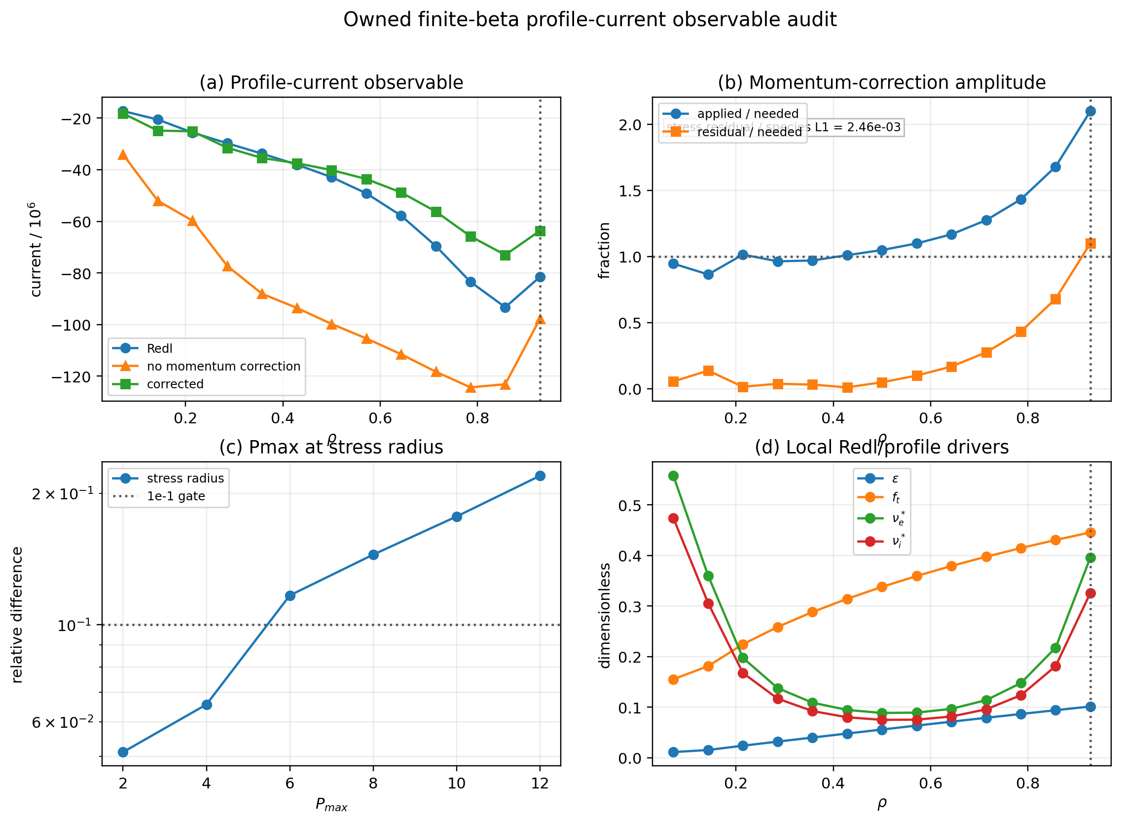
python examples/owned_finite_beta_profile_current_observable_audit.py
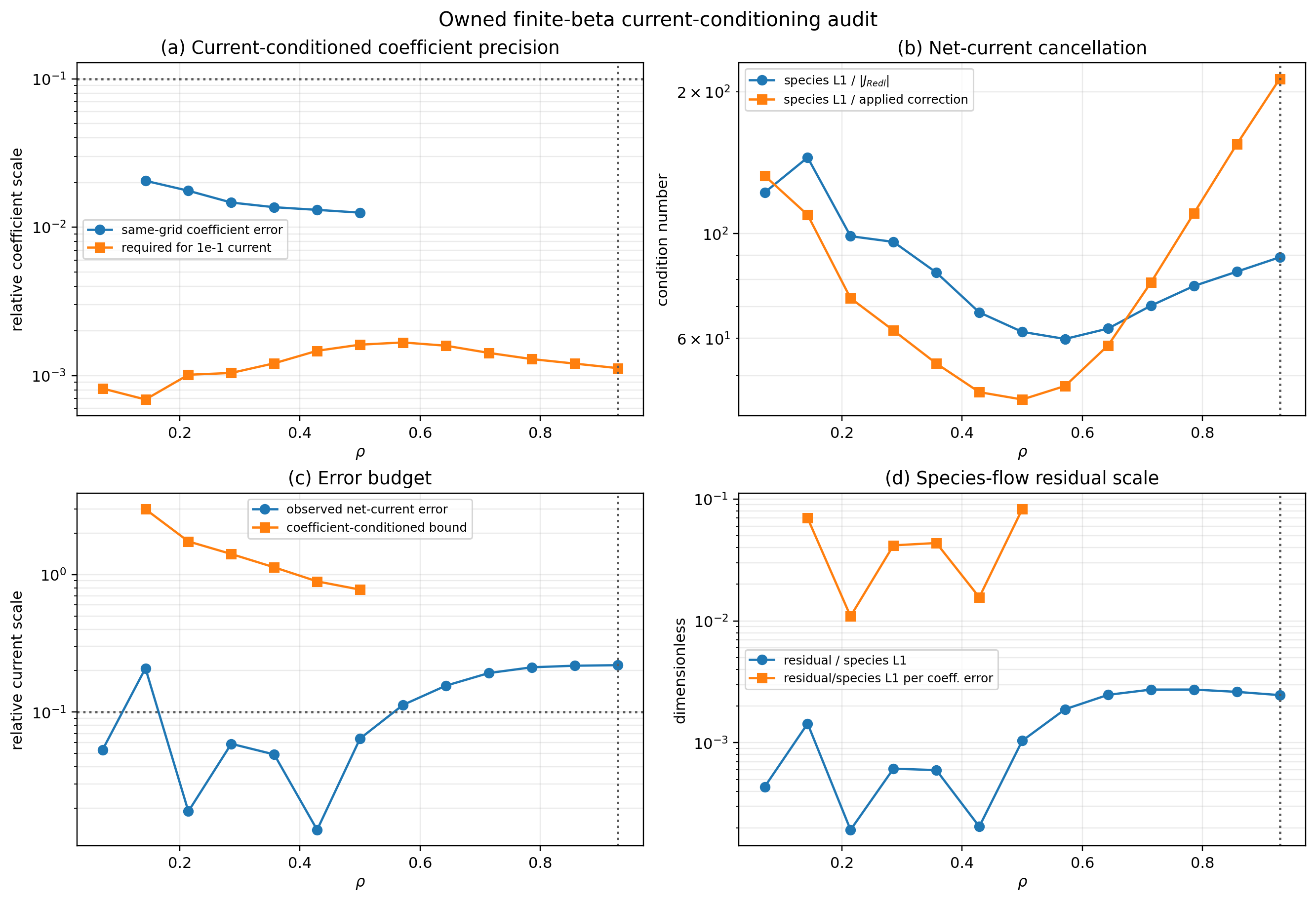
python examples/owned_finite_beta_current_conditioning_audit.py
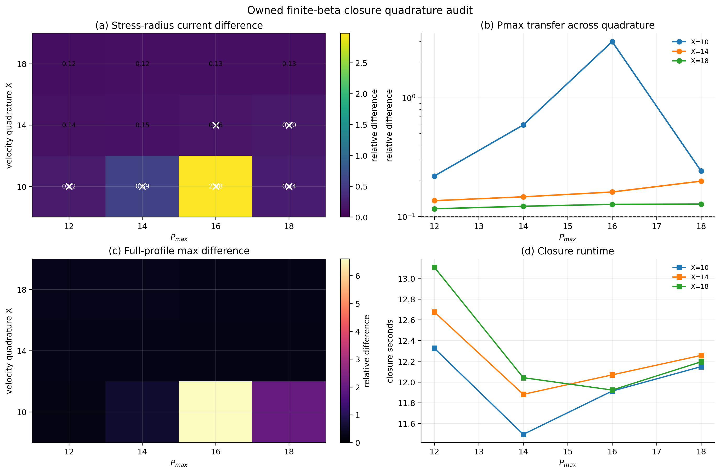
python examples/owned_finite_beta_closure_quadrature_audit.py
python examples/owned_finite_beta_source_channel_audit.py
python examples/owned_finite_beta_source_response_profile_audit.py
python examples/owned_finite_beta_radial_interpolation_audit.py --rebuild-matched
python examples/owned_finite_beta_closure_quadrature_audit.py \
--bootstrap-json docs/_static/owned_finite_beta_field_radius_matched_bootstrap_comparison.json \
--x-values 10 18 --n-orders 10 12 14 18 \
--output-prefix docs/_static/owned_finite_beta_field_radius_matched_closure_quadrature_audit \
--output-dir examples/outputs/owned_finite_beta_field_radius_matched_quadrature_probe
python examples/owned_finite_beta_source_channel_audit.py \
--bootstrap-json docs/_static/owned_finite_beta_field_radius_matched_bootstrap_comparison.json \
--settings 10:12 10:18 18:18 \
--output-prefix docs/_static/owned_finite_beta_field_radius_matched_source_channel_audit \
--output-dir examples/outputs/owned_finite_beta_field_radius_matched_quadrature_probe
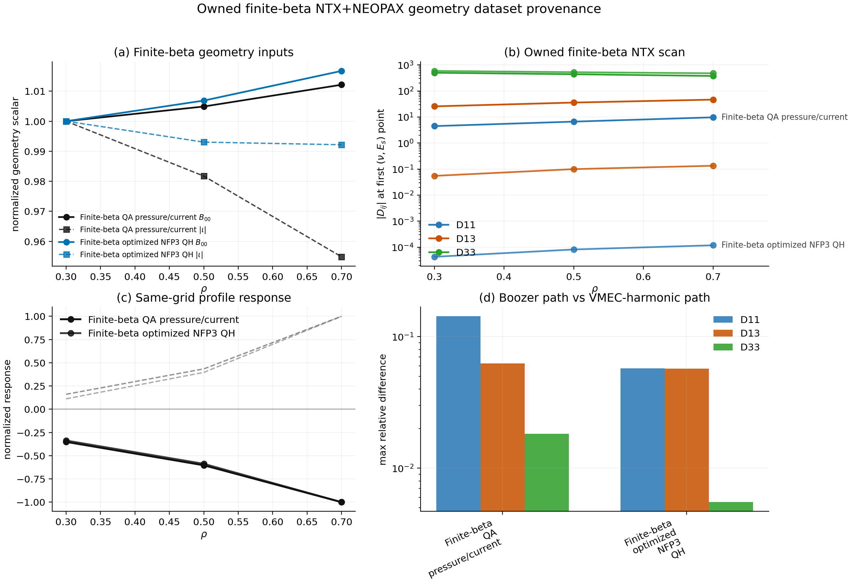
These optional provenance artifacts prioritize local finite-beta stellarator
input/wout pairs. The NTX/NEOPAX script builds finite-beta QA surfaces through
vmex -> booz_xform_jax with the physical VMEC edge-flux scale passed
explicitly as psi_p, writes NEOPAX-style HDF5 scan tables, stores compact
profile flux/current proxies from those same tables, and compares that path
with the direct VMEC-harmonic interpolation path on the same radial and
collisionality grid. Optimized finite-beta QH/QI cases are retained as direct
wout-harmonic stress cases until their current-profile representation is
supported by the JAX geometry stack.
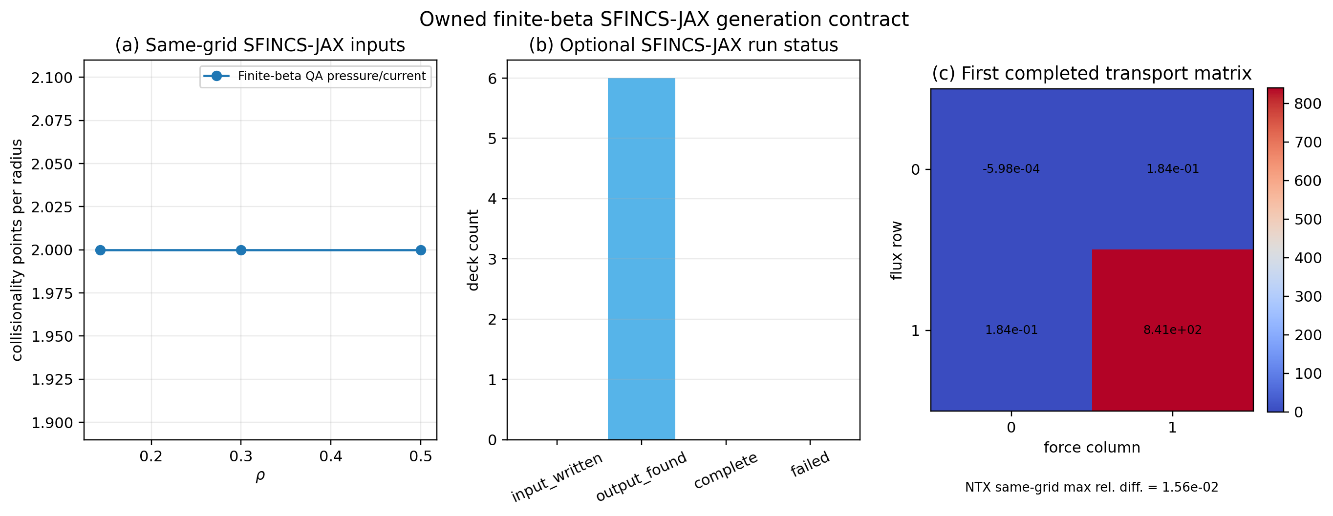
The SFINCS-JAX script writes owned RHSMode=3 input decks for the same
finite-beta wout, rho, collisionality, electric-field, and resolution
contract. Use --run-sfincs-jax for explicit local runs; completed HDF5
outputs are ingested into the JSON sidecar with the SFINCS-reported
nuPrime -> nu_n bridge and a coefficient-level NTX L13/L31/L33
comparison. The committed artifact now contains a six-point same-grid
finite-beta QA ladder; use it as a smoke-resolution transport-coefficient
localization tool, not as a bootstrap-current parity claim.
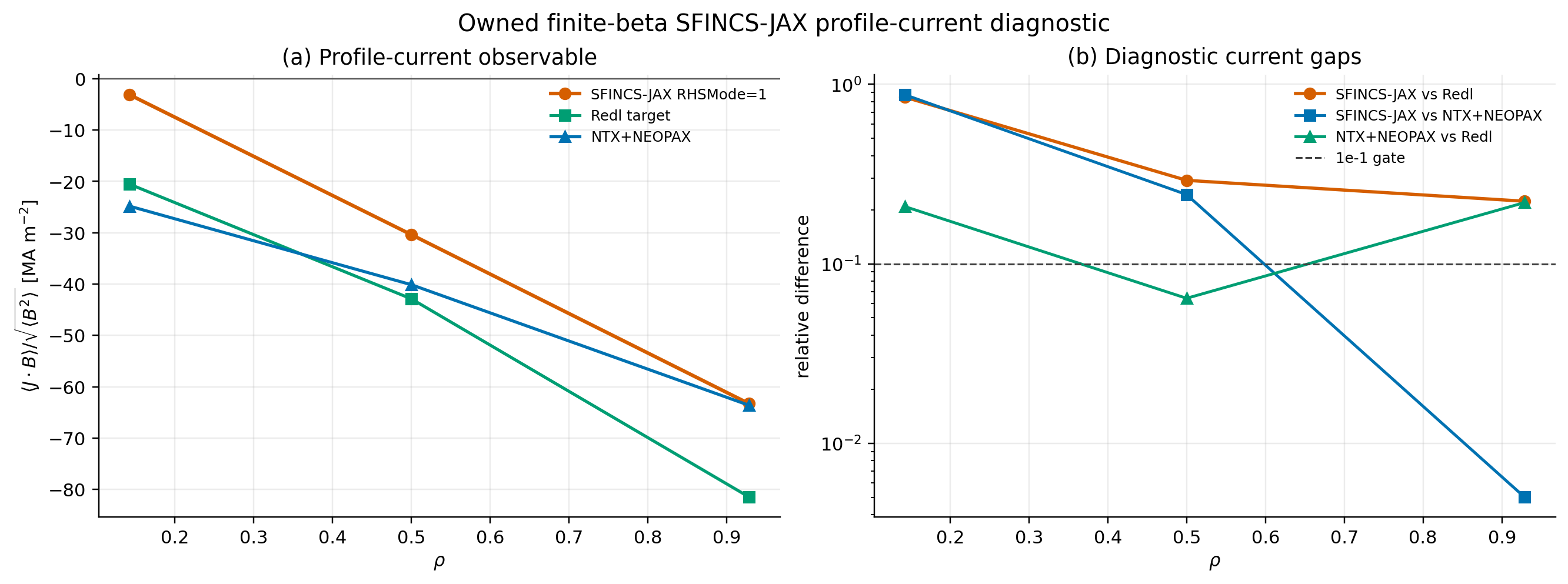
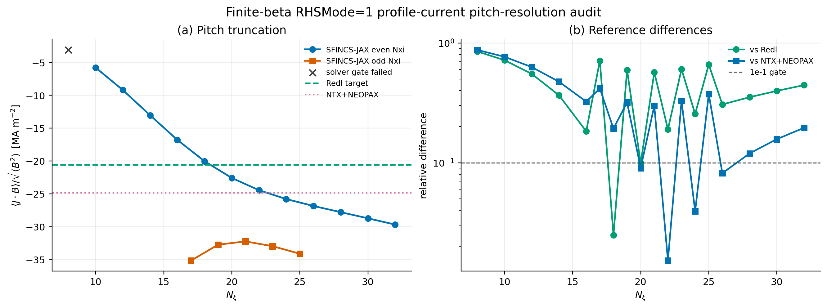
The RHSMode=1 profile-current diagnostic uses the same finite-beta VMEC wout,
analytic profiles, current observable, and Redl/NTX+NEOPAX comparison
contract. The committed low-resolution artifact is a direct-profile
normalization and convergence diagnostic. Its high-Nxi even/odd pitch gap is
accepted at 1.32e-1 under the 1.5e-1 reduced-closure stress tolerance.
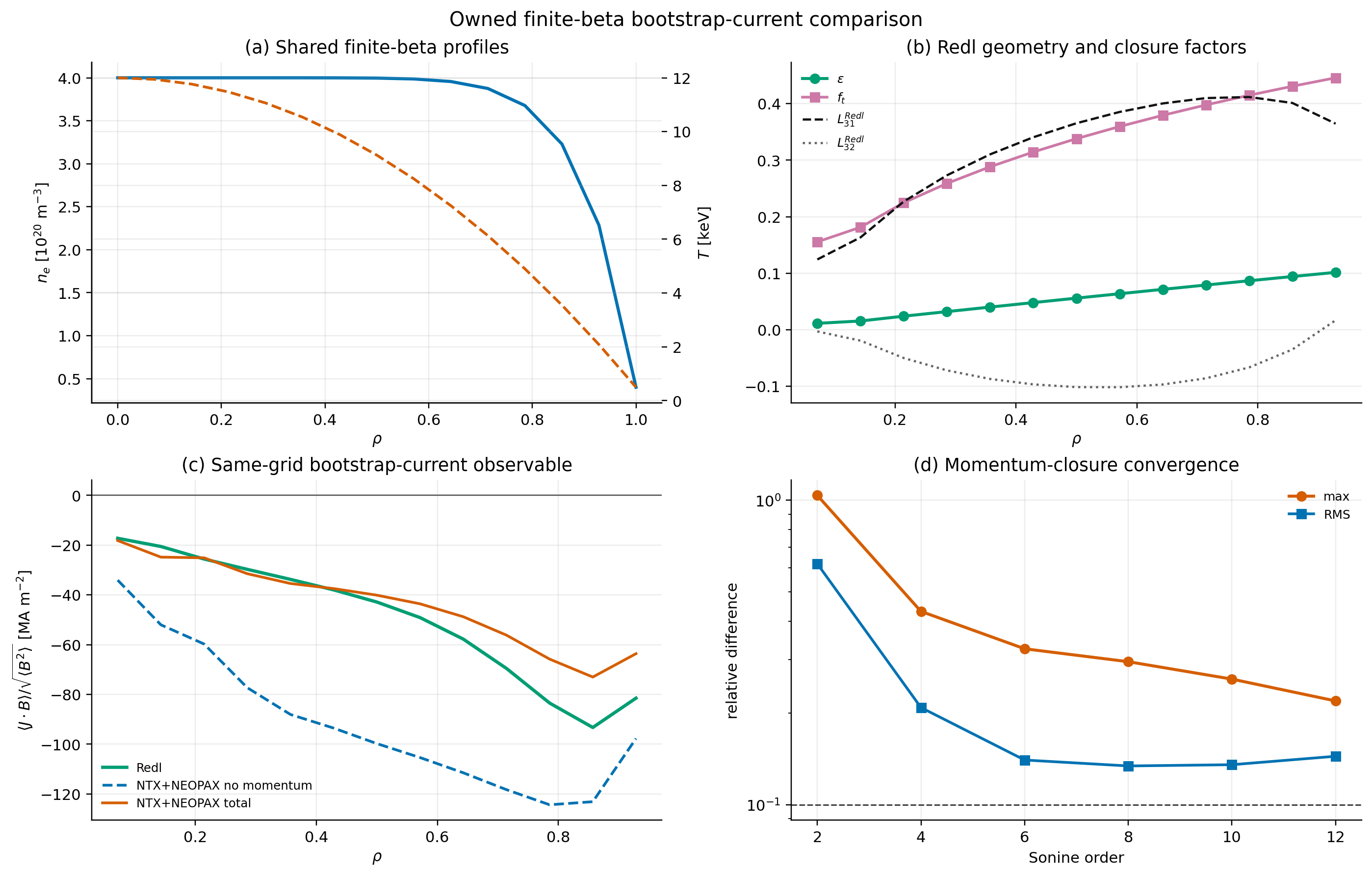
The finite-beta bootstrap-current script runs Redl and NTX+NEOPAX on the
same QA pressure/current wout, Boozer transform, analytic profile contract,
radial grid, adaptive physical nu/v support, and current normalization. It
uses the normalized-radius Boozer B00(rho) convention, including
dB00/dr = (dB00/d rho)/a_b, so the file-backed field object and the profile
closure use the same radial coordinate. It is a production-resolution
reduced-closure stress audit for this QA case; the current JSON sidecar records
the remaining profile-wide Redl/NTX+NEOPAX residual and a Sonine-order
convergence scan instead of promoting the figure as parity.
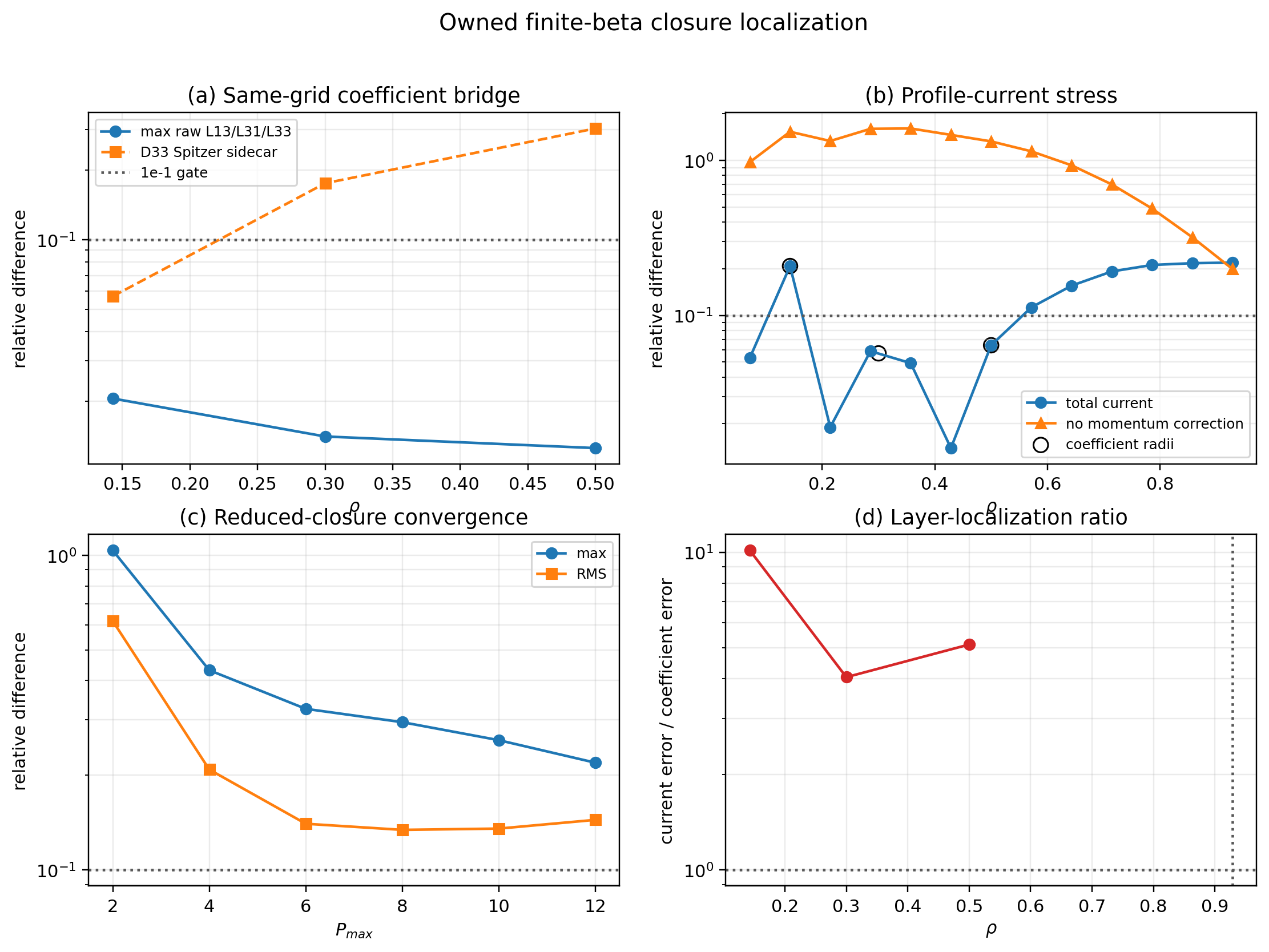
The closure-localization script then overlays these two committed sidecars. It
shows that the same-grid L13/L31/L33 coefficient ladder remains below the
coefficient gate, while the profile-current residual is still larger than the
1e-1 current gate; the non-promoted follow-up is therefore the reduced
profile-current observable rather than the monoenergetic coefficient bridge.
The profile-current observable audit decomposes the same stress radius into the
no-momentum current, applied momentum correction, correction needed to match the
Redl target, Pmax trend, species-current cancellation scale, and local
profile/geometry drivers.
The current-conditioning audit then asks a stricter question: given the observed
electron/ion cancellation, how accurate must the same-grid coefficient ladder be
before coefficient uncertainty can be ruled out for a 1e-1 net-current gate?
For the current finite-beta QA artifact, the stress radius needs about
1.1e-3 coefficient precision, while the completed coefficient ladder is still
order 2e-2. That keeps the next step focused on production-resolution
same-grid coefficient/profile-current diagnostics before any closure change is
promoted.
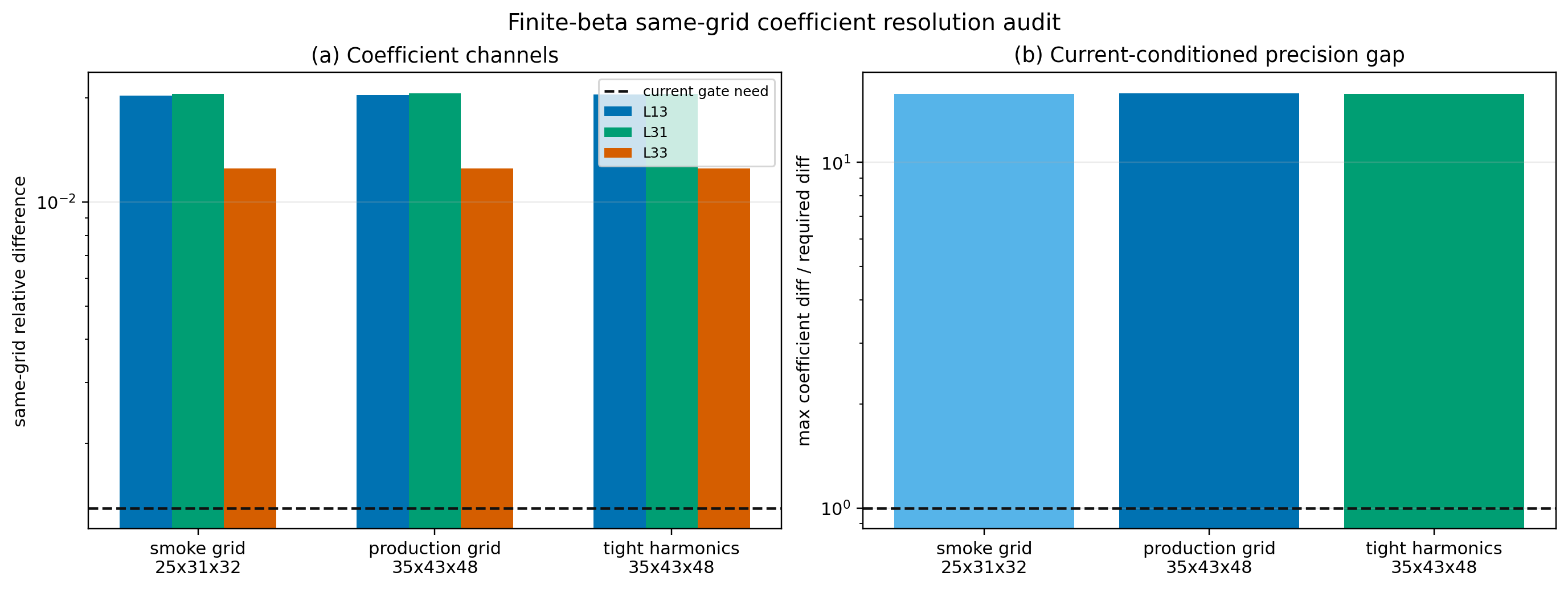
The resolution audit adds the first production stress probe: increasing the
same point to 35 x 43 x 48 and tightening the VMEC harmonic cutoff leaves the
coefficient floor near 2.05e-2, so the remaining finite-beta current gap is
not explained by those numerical knobs.
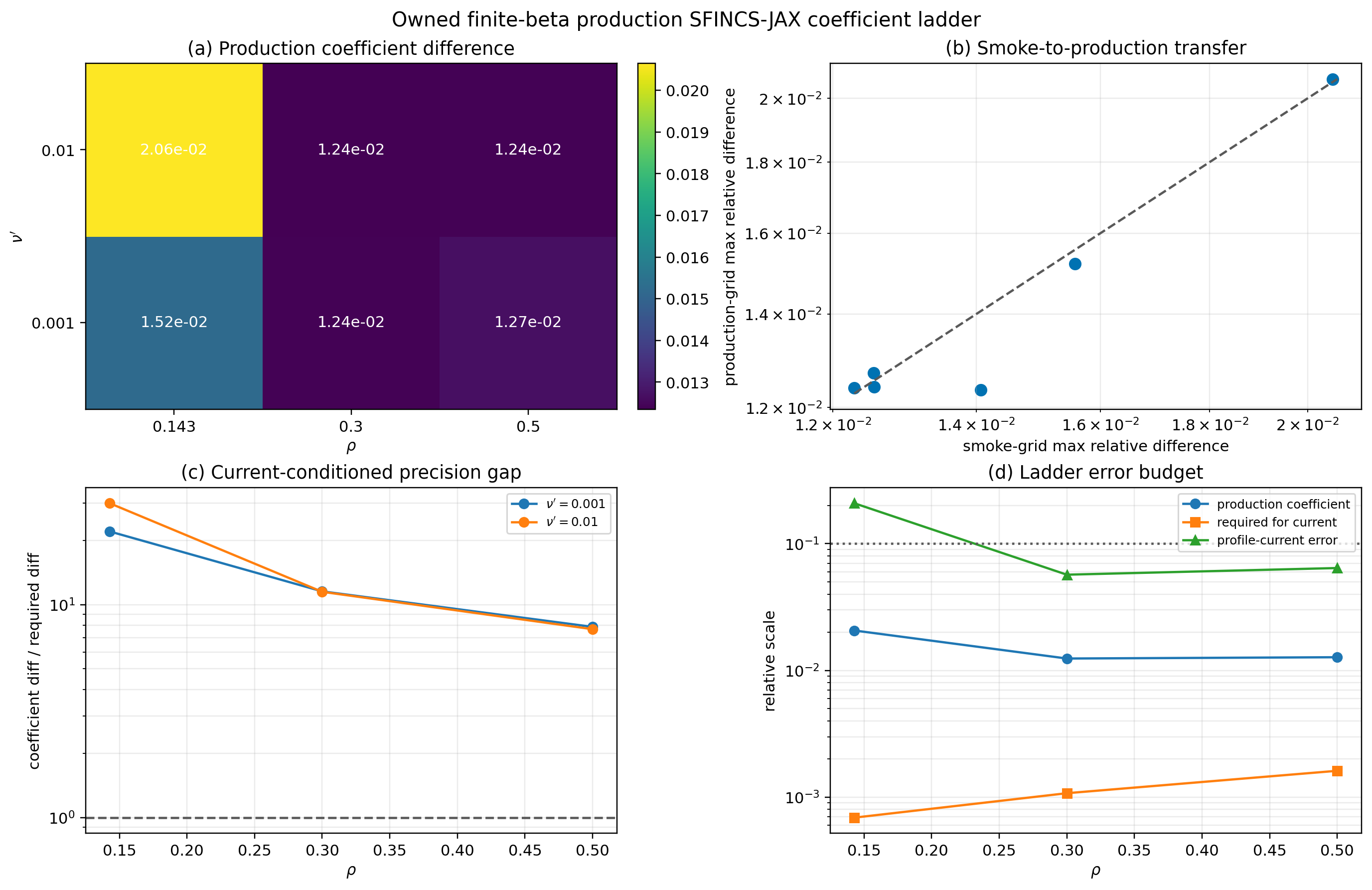
The production-ladder audit then reads the six production same-grid
SFINCS-JAX points across the owned finite-beta QA radii and collisionalities.
All completed coefficient differences stay below 2.07e-2; the
current-conditioned precision gap remains larger than the coefficient floor, so
the next open item is the profile-current closure observable.
The closure-quadrature audit holds the same scan, Redl observable, profiles, and
normalization fixed while varying only Sonine order and velocity quadrature.
After the Boozer-field normalization fix, it records no stress-radius current
gate pass; the best stress point remains above 1e-1 and the full-profile
maximum remains a monitored reduced-closure residual.
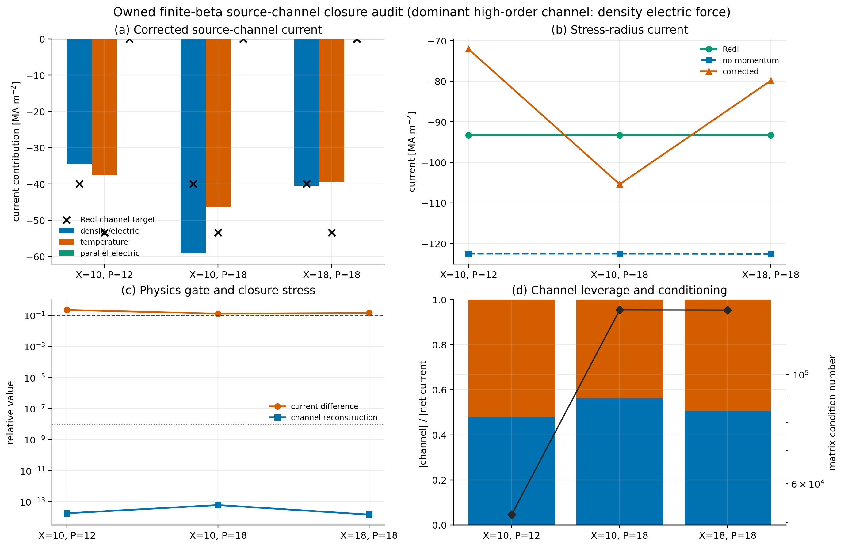
The source-channel audit then freezes the same momentum-restoring matrix and
solves one physical source channel at a time. The one-channel solves reconstruct
the corrected current to roundoff. The corrected high-order stress is a mixed
density/electric and temperature-gradient response with no parallel-electric
drive for this profile contract.
The profile source-response audit extends that decomposition from the single
stress radius to the full finite-beta profile at X=18, P=18. It plots the
Redl and corrected current profiles, the Redl/NTX effective source-response
multiplier, the reconstruction gate, and the response trend against Redl
collisionality and trapped-particle fraction. This is a diagnostic for the next
physics closure, not a fitted runtime correction.
The closure-target audit reads that profile-response artifact and ranks local
drivers before a runtime model is proposed. The current sidecar selects the
Redl geometry factor epsilon as the strongest single driver and records that
the best diagnostic model is not applied to the code.
The radial-interpolation audit rebuilds the same current observable on the
field radii. It changes individual radii but does not improve the full-profile
maximum; the matched-radius quadrature rerun still finds zero quadrature-stable
current-gate passes.
The matched-radius source-channel rerun reconstructs the corrected current to
roundoff and shows the same pattern: X=18, P=18 remains a quadrature-stable
source-response stress diagnostic rather than a finite-beta parity claim.
It writes:
docs/_static/owned_geometry_neopax_dataset.pngdocs/_static/owned_geometry_neopax_dataset.pdfdocs/_static/owned_geometry_neopax_dataset.jsondocs/_static/owned_geometry_neopax_database/*.h5docs/_static/owned_finite_beta_sfincs_jax_inputs.pngdocs/_static/owned_finite_beta_sfincs_jax_inputs.pdfdocs/_static/owned_finite_beta_sfincs_jax_inputs.jsondocs/_static/owned_finite_beta_sfincs_jax_resolution_audit.pngdocs/_static/owned_finite_beta_sfincs_jax_resolution_audit.pdfdocs/_static/owned_finite_beta_sfincs_jax_resolution_audit.jsondocs/_static/owned_finite_beta_sfincs_jax_production_ladder.pngdocs/_static/owned_finite_beta_sfincs_jax_production_ladder.pdfdocs/_static/owned_finite_beta_sfincs_jax_production_ladder.jsondocs/_static/owned_finite_beta_sfincs_jax_production_ladder_audit.pngdocs/_static/owned_finite_beta_sfincs_jax_production_ladder_audit.pdfdocs/_static/owned_finite_beta_sfincs_jax_production_ladder_audit.jsondocs/_static/owned_finite_beta_sfincs_jax_profile_current_audit.pngdocs/_static/owned_finite_beta_sfincs_jax_profile_current_audit.pdfdocs/_static/owned_finite_beta_sfincs_jax_profile_current_audit.jsondocs/_static/owned_finite_beta_sfincs_jax_profile_current_resolution_audit.pngdocs/_static/owned_finite_beta_sfincs_jax_profile_current_resolution_audit.pdfdocs/_static/owned_finite_beta_sfincs_jax_profile_current_resolution_audit.jsonexamples/outputs/owned_finite_beta_sfincs_jax_inputs/**/input.namelistdocs/_static/owned_finite_beta_bootstrap_comparison.pngdocs/_static/owned_finite_beta_bootstrap_comparison.pdfdocs/_static/owned_finite_beta_bootstrap_comparison.jsondocs/_static/owned_finite_beta_closure_localization.pngdocs/_static/owned_finite_beta_closure_localization.pdfdocs/_static/owned_finite_beta_closure_localization.jsondocs/_static/owned_finite_beta_profile_current_observable_audit.pngdocs/_static/owned_finite_beta_profile_current_observable_audit.pdfdocs/_static/owned_finite_beta_profile_current_observable_audit.jsondocs/_static/owned_finite_beta_current_conditioning_audit.pngdocs/_static/owned_finite_beta_current_conditioning_audit.pdfdocs/_static/owned_finite_beta_current_conditioning_audit.jsondocs/_static/owned_finite_beta_closure_quadrature_audit.pngdocs/_static/owned_finite_beta_closure_quadrature_audit.pdfdocs/_static/owned_finite_beta_closure_quadrature_audit.jsondocs/_static/owned_finite_beta_source_channel_audit.pngdocs/_static/owned_finite_beta_source_channel_audit.pdfdocs/_static/owned_finite_beta_source_channel_audit.jsondocs/_static/owned_finite_beta_source_response_profile_audit.pngdocs/_static/owned_finite_beta_source_response_profile_audit.pdfdocs/_static/owned_finite_beta_source_response_profile_audit.jsondocs/_static/owned_finite_beta_closure_target_audit.pngdocs/_static/owned_finite_beta_closure_target_audit.pdfdocs/_static/owned_finite_beta_closure_target_audit.jsondocs/_static/owned_finite_beta_radial_interpolation_audit.pngdocs/_static/owned_finite_beta_radial_interpolation_audit.pdfdocs/_static/owned_finite_beta_radial_interpolation_audit.jsondocs/_static/owned_finite_beta_field_radius_matched_bootstrap_comparison.jsondocs/_static/owned_finite_beta_field_radius_matched_closure_quadrature_audit.pngdocs/_static/owned_finite_beta_field_radius_matched_closure_quadrature_audit.pdfdocs/_static/owned_finite_beta_field_radius_matched_closure_quadrature_audit.jsondocs/_static/owned_finite_beta_field_radius_matched_source_channel_audit.pngdocs/_static/owned_finite_beta_field_radius_matched_source_channel_audit.pdfdocs/_static/owned_finite_beta_field_radius_matched_source_channel_audit.jsonexamples/outputs/owned_finite_beta_bootstrap_comparison/*.h5
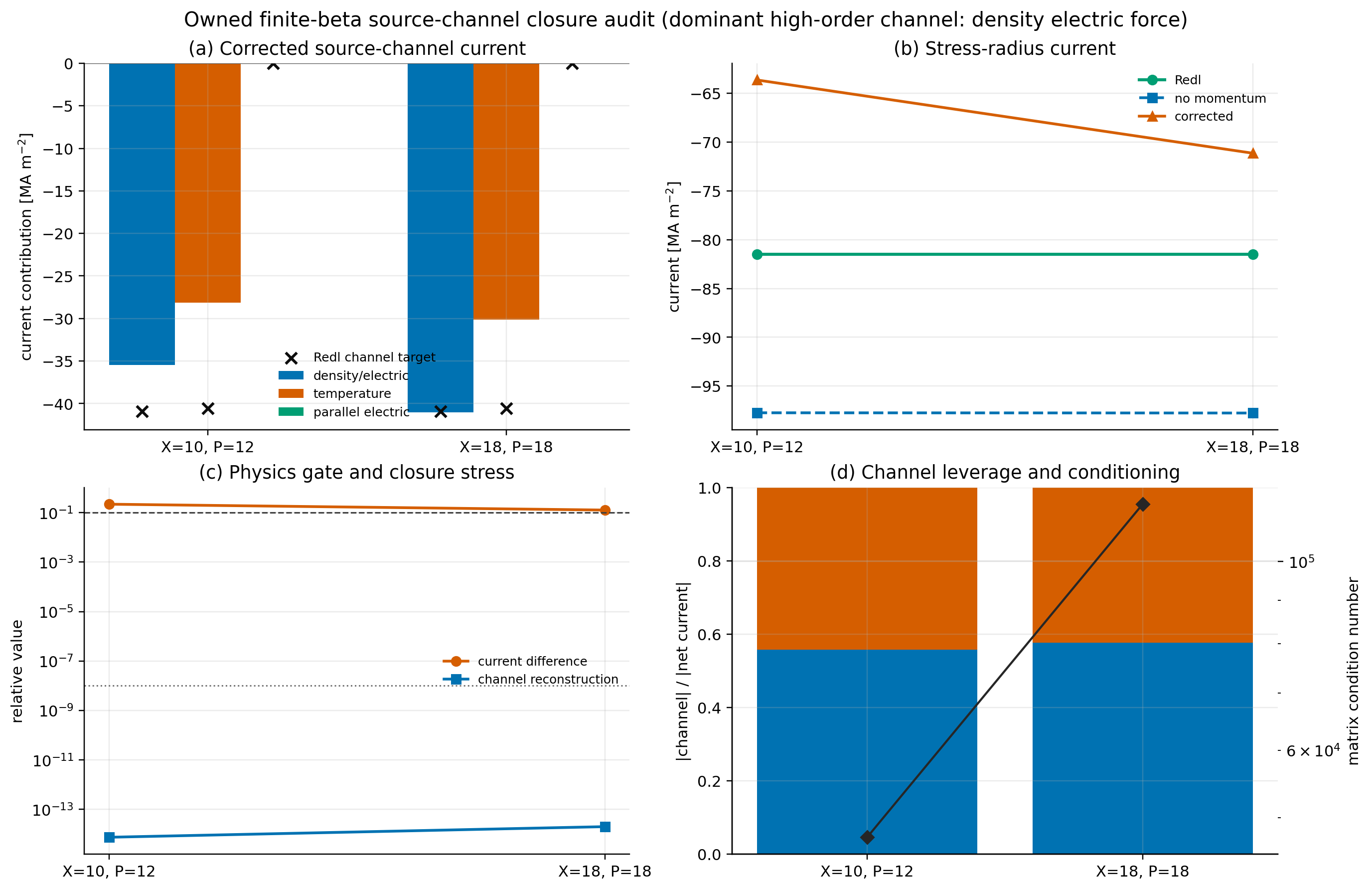
The source-channel panel overlays the Redl density and temperature target terms on the same current observable. The current artifact reconstructs the corrected NTX+NEOPAX current to roundoff and records a mixed density/electric and temperature-gradient high-order stress response.
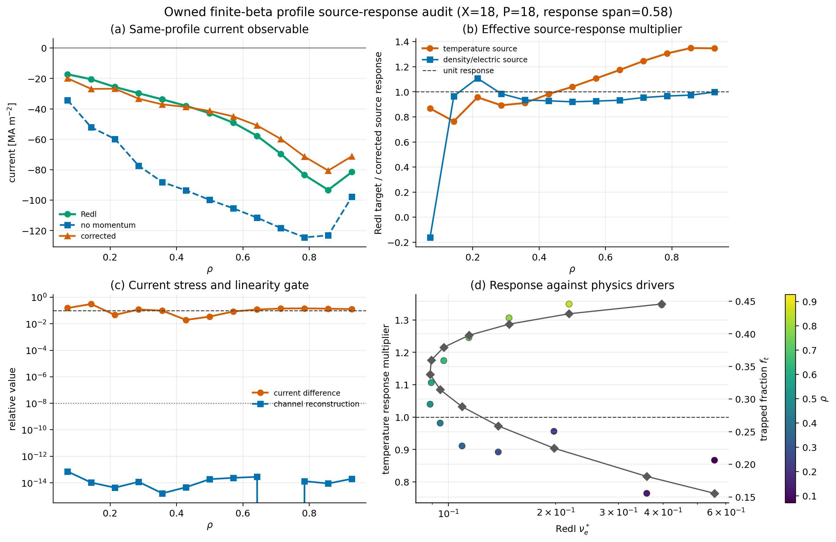
The profile source-response panel shows that the temperature response multiplier is not a single hidden constant: it spans the profile while preserving source sign agreement, with the high-order stress largest at the inner radius.
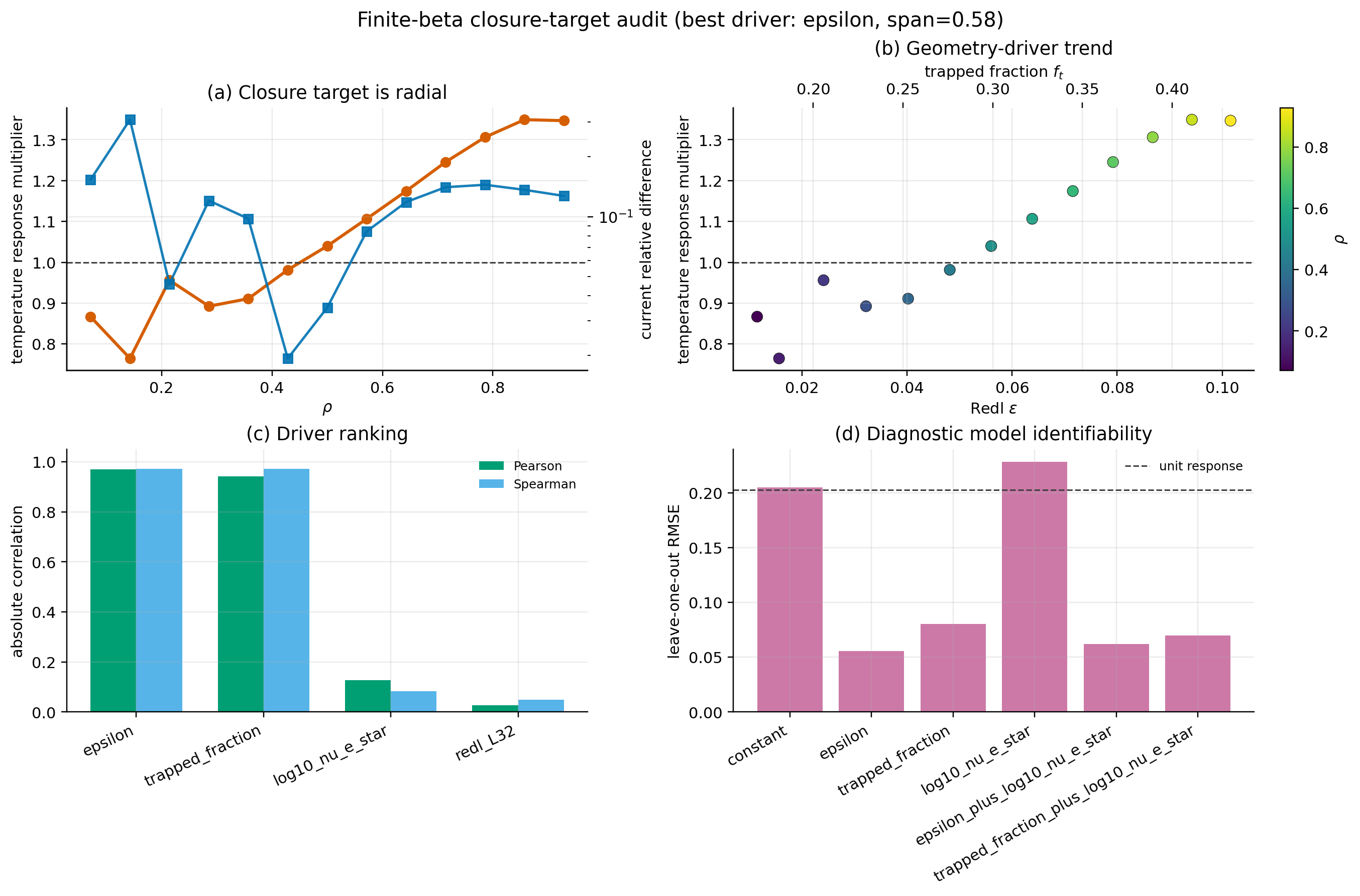
The closure-target panel ranks geometry, trapped-particle, and collisionality drivers for the measured response. It is a model-identification artifact only: the runtime closure remains unchanged until a physics-derived term passes the fixed-field, W7-X transfer, source reconstruction, and same-grid finite-beta coefficient gates. Its JSON sidecar also cross-links the field-radius-matched source-channel and quadrature artifacts, confirming that the matched audit uses the same stress radius, reconstructs the source response, and still has no quadrature-stable current-gate pass.
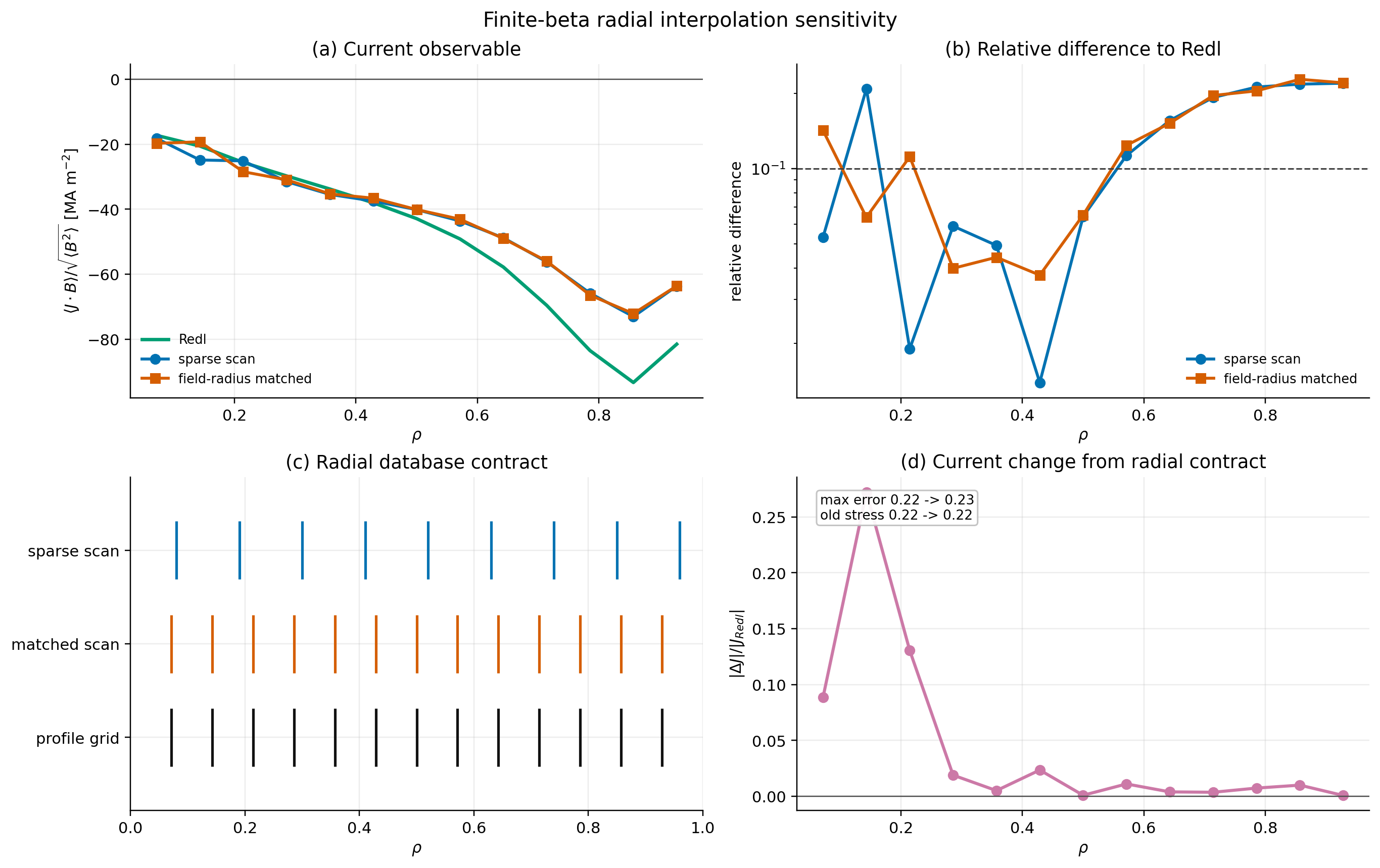
The radial-interpolation panel rebuilds the same finite-beta current audit with the monoenergetic database placed on the exact profile-current field radii. It changes individual radii but does not clear the full-profile current gate, so no runtime interpolation policy is promoted.
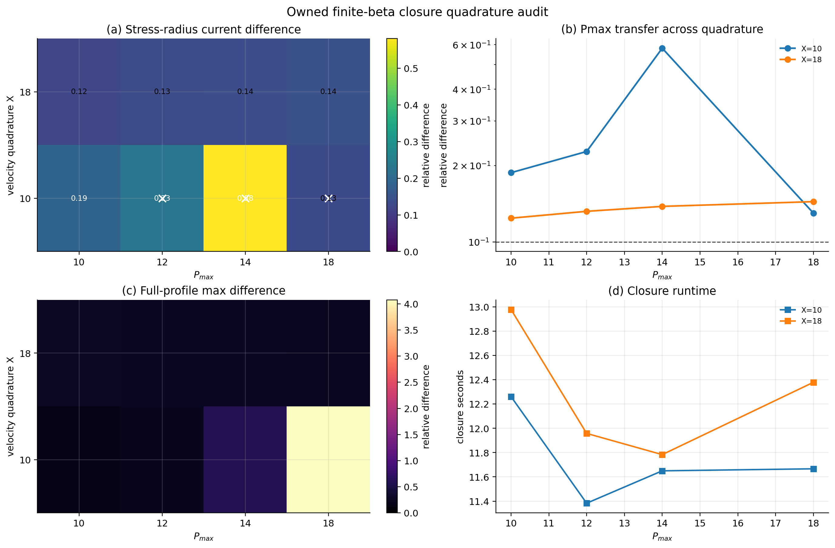
The matched closure-quadrature panel repeats the Sonine/quadrature sweep after removing the sparse-radius interpolation layer. It still has zero quadrature-stable current-gate passes, so the non-promoted follow-up remains a quadrature-stable reduced profile-current closure.
The matched source-channel panel repeats the physical RHS decomposition on the same field-radius-matched contract. It reconstructs the corrected current to roundoff and keeps the remaining finite-beta mismatch localized to a quadrature-stable source-response stress.
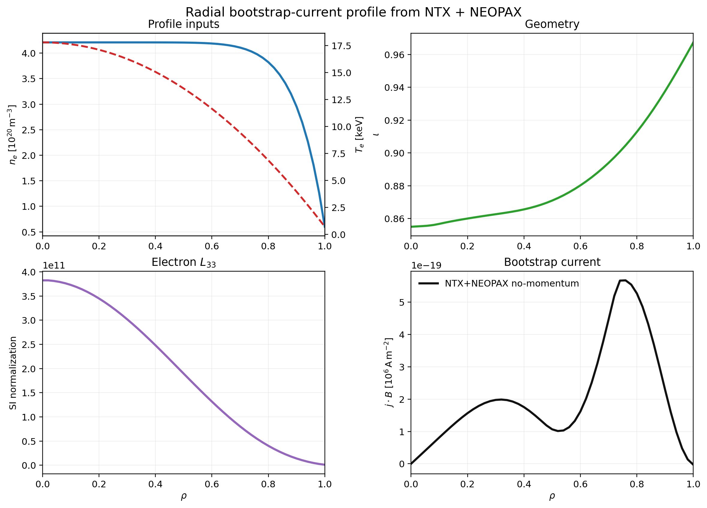
12. Bootstrap Current With NEOPAX
python examples/bootstrap_current_with_neopax.py
This is the shortest user-facing NTX + NEOPAX radial-profile workflow. It:
loads the W7-X reference equilibrium from the local NEOPAX checkout
builds an NTX monoenergetic scan on the archived
(\rho, \nu_v, E_r)axesmaps that scan into NEOPAX monoenergetic arrays
evaluates the bootstrap-current profile with the no-momentum closure
optionally overlays the momentum-correction branch
It writes:
docs/_static/bootstrap_current_with_neopax.pngdocs/_static/bootstrap_current_with_neopax.pdfdocs/_static/bootstrap_current_with_neopax.json
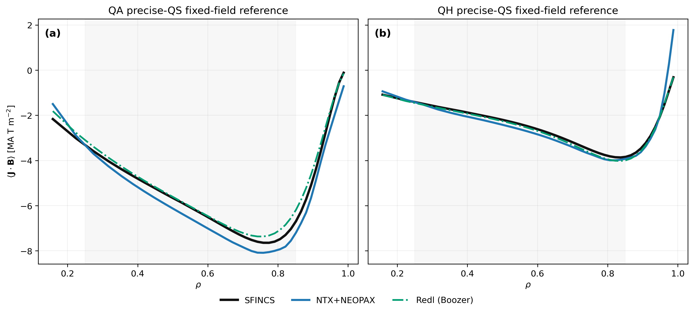
13. Fixed-Field Bootstrap-Current Validation
python examples/bootstrap_current_fixed_field_validation.py
This local archive-backed benchmark compares:
archived Fortran SFINCS
SFINCS-JAX reruns of the archived inputs
Redl on the same precise-QS QA/QH reference family
NTX+NEOPAXon the same equilibria and archived profiles
It writes:
docs/_static/bootstrap_current_fixed_field_validation.pngdocs/_static/bootstrap_current_fixed_field_validation.pdfdocs/_static/bootstrap_current_fixed_field_validation.json
Use this script for the fixed-field validation figure that is shown in the
README. The figure intentionally overlays only bootstrap-current profiles; the
interior-window relative-error gates are stored in the JSON artifact and checked
by the physics-gate tests. The current artifact keeps both the Redl analytic
comparison and the reduced NTX+NEOPAX total-current stress comparison below
the 1e-1 gate.
14. Autodiff Inverse Problem
python examples/autodiff_inverse_problem.py
This writes docs/_static/autodiff_inverse_problem.{png,pdf} and demonstrates
recovery of a Boozer harmonic from synthetic transport data using JAX
gradients.
15. Precise-QS Redl Versus SFINCS Audit
python examples/precise_qs_redl_sfincs_audit.py
This local archive-backed audit uses the fixed-field Landreman–Paul QA/QH reference family from the Zenodo bundle and writes:
examples/outputs/precise_qs_redl_sfincs_audit/precise_qs_redl_sfincs_audit.pngexamples/outputs/precise_qs_redl_sfincs_audit/precise_qs_redl_sfincs_audit.pdfexamples/outputs/precise_qs_redl_sfincs_audit/precise_qs_redl_sfincs_audit.json
It compares the archived SFINCS bootstrap-current profiles against:
Redl with the VMEC-side trapped-fraction path
Redl with a Boozer-side trapped-fraction path reconstructed through
booz_xform_jax
Use this script when auditing the analytic fixed-field benchmark itself, not
the integrated NTX+NEOPAX workflow. The plot is an overlay-only
bootstrap-current comparison; the relative-error metrics remain in the JSON
artifact.
16. Fixed-Field Transport-Matrix Audit
python examples/fixed_field_transport_matrix_audit.py
This local audit writes:
examples/outputs/fixed_field_transport_matrix_audit/fixed_field_transport_matrix_audit.pngexamples/outputs/fixed_field_transport_matrix_audit/fixed_field_transport_matrix_audit.pdfexamples/outputs/fixed_field_transport_matrix_audit/fixed_field_transport_matrix_audit.json
It runs SFINCS-JAX in RHSMode=3 on the same fixed-field QA/QH reference
family and compares L13, L31, and L33 against NTX candidate channels.
This audit now:
reproduces the exact SFINCS
RHSMode=3monoenergetic overwrite fornu_nuses archive-backed Landreman/H. Smith bridge factors for the
L13/L31/L33channelsnarrows the remaining blocker to the
L33bridge rather than a generic sign or family-selection problem
This is still the coefficient-side gate for the public NTX+NEOPAX
bootstrap-current validation figure.
17. Autodiff Derivative Audit
python examples/derivative_audit.py
This writes docs/_static/derivative_audit.{png,pdf} and compares direct JAX
gradients of the dense solve against centered finite differences for:
D11andD33sensitivities to a Boozer harmonic amplitudeD11andD33sensitivities to the radial electric field
This is the validation baseline for the current prepared implicit-adjoint derivative implementation.
18. Prepared-Derivative Benchmark
python examples/derivative_path_benchmark.py
This writes docs/_static/derivative_path_benchmark.{png,pdf} and compares:
direct reverse-mode through
solve_prepared_coefficient_vector(...)selective recomputation through
jax.checkpoint(...)the prepared custom-VJP path through
solve_prepared_coefficient_vector_vjp(...)forward mode and centered finite differences
The artifact reports synchronized runtime, XLA temporary memory, independent full primal/transpose residuals, and derivative agreement. A low-collisionality point that agrees across derivative methods but fails the primal residual gate is retained as an explicit non-certified case.
It also writes docs/_static/derivative_path_benchmark.json for manuscript
tables and reproducibility notes.
19. Autodiff NEOPAX Profiles
python examples/neopax_autodiff_profiles.py
This writes docs/_static/autodiff_neopax_profiles.{png,pdf} and demonstrates
a low-dimensional electric-field profile inversion on NEOPAX-style
monoenergetic arrays.
20. Autodiff Profile Uncertainty
python examples/autodiff_profile_uncertainty.py
This writes docs/_static/autodiff_profile_uncertainty.{png,pdf,json} and
compares linearized covariance propagation against a small Monte Carlo ensemble
for the differentiable NEOPAX-style profile fit under a prescribed Gaussian
parameter perturbation.
21. Robust Bootstrap-Current Optimization
python examples/bootstrap_current_robust_optimization.py
This writes docs/_static/bootstrap_current_robust_optimization.{png,pdf,json}
and compares deterministic versus robust optimization of the scalar
bootstrap-current response under a prescribed Gaussian control uncertainty.
22. Ambipolar Profile
python examples/ambipolar_profile.py
This writes:
docs/_static/ambipolar_profile.pngdocs/_static/ambipolar_profile.pdf
and demonstrates:
building a radial NTX scan from explicit in-memory surfaces
defining two species profiles with
A1(r),A3(r), and\nu_v(r)visualizing the residual landscape over the scanned
E_raxissolving a smooth ambipolar
E_r(r)profile with radial regularizationevaluating the resulting reduced bootstrap-current response profile
23. Ambipolar Profile Family
python examples/ambipolar_profile_family.py
This writes:
docs/_static/ambipolar_profile_family.pngdocs/_static/ambipolar_profile_family.pdf
and demonstrates:
solving a small family of ambipolar closures on one NTX radial scan
comparing the integrated residual landscapes across explicit profile controls
evaluating a bootstrap-current objective across that family
selecting the best control point from a scalar objective landscape
24. Science Case: Bootstrap-Current Optimization
python examples/bootstrap_current_optimization.py
This writes docs/_static/bootstrap_current_optimization.{png,pdf} and shows a
differentiable geometry-control problem:
a VMEC-derived radial surface family
one dominant non-axisymmetric harmonic used as the control variable
autodiff optimization of a weighted bootstrap-current response
explicit serial-versus-multiprocess timing annotations
This is the main application/science-case figure for a methods paper centered on bootstrap-current analysis and optimization.
It also writes docs/_static/bootstrap_current_optimization.json for the
manuscript table builder.
25. Profile-Control Optimization
python examples/profile_control_optimization.py
This writes:
docs/_static/profile_control_optimization.pngdocs/_static/profile_control_optimization.pdf
and demonstrates:
building a differentiable scalar control on top of the profile closure
optimizing that control directly against a bootstrap-current objective
reusing the ambipolar solve inside a JAX optimization loop
26. Profile-Basis Optimization
python examples/profile_basis_optimization.py
This writes:
docs/_static/profile_basis_optimization.pngdocs/_static/profile_basis_optimization.pdf
and demonstrates:
using a small radial basis to perturb the profile closure
optimizing several control amplitudes simultaneously
retaining a compact, publication-grade figure for a higher-dimensional optimization workflow
27. Profile Transport Loop
python examples/profile_transport_loop.py
This writes:
docs/_static/profile_transport_loop.pngdocs/_static/profile_transport_loop.pdf
and demonstrates:
iterating a simple self-consistent profile closure on top of the ambipolar solve
updating
A1(r)andA3(r)directly from transport mismatchestracking accepted-step transport-loss descent together with the ambipolar closure
smoothing the updated force profiles radially before the next ambipolar solve
28. Primitive Profile Transport
python examples/primitive_profile_transport.py
This writes:
docs/_static/primitive_profile_transport.pngdocs/_static/primitive_profile_transport.pdf
and demonstrates:
reconstructing
A1(r)andA3(r)from primitive density and temperature profilescomparing initial and final residual/current profiles for the primitive closure
updating density and temperature instead of thermodynamic-force channels directly
enforcing explicit density/temperature source-target closure terms in addition to the transport mismatch
exposing the derived monoenergetic force profiles alongside the final primitive state
29. Performance Scaling
python examples/performance_scaling.py --cpu-json ... --gpu-json ...
This writes publication-style CPU/GPU scaling figures from benchmark JSON payloads.
30. Prepared-Geometry Reuse Profile
python examples/prepared_geometry_reuse_profile.py --preset paper
This writes:
docs/_static/prepared_geometry_reuse_profile.pngdocs/_static/prepared_geometry_reuse_profile.pdfdocs/_static/prepared_geometry_reuse_profile.json
and profiles direct repeated solves, prepared geometry reuse, and a compiled prepared solver on one fixed geometry. It is a performance artifact for optimization workflows, not a physics-parity claim.
31. Profile Force Reconstruction Audit
python examples/profile_force_reconstruction_audit.py
This writes:
docs/_static/profile_force_reconstruction_audit.pngdocs/_static/profile_force_reconstruction_audit.pdfdocs/_static/profile_force_reconstruction_audit.json
and validates the primitive-profile reconstruction path against the archived
precise-QS QA/QH benchmark family by comparing NTX-reconstructed A1(\rho) and
A3(\rho) against the exact derivatives implied by the archived density,
temperature, and normalized electric-field inputs. This is a monitored
benchmark-family stress test for the current primitive-profile builder, not a
parity claim.
32. Validation Summary
python examples/validation_summary.py
This writes:
docs/_static/validation_summary.pngdocs/_static/validation_summary.pdfdocs/_static/validation_summary.json
It is the recommended core validation figure for a methods paper because it combines transport trends, Onsager closure, and Legendre convergence on the same DKES-style and VMEC benchmark surfaces. This benchmark is anchored to the monoenergetic convergence/benchmarking literature of Escoto et al. 2024 and to the low-collisionality regime discussion of Helander, Parra, and Newton 2017.
The JSON sidecar freezes the plotted curves, low-collisionality tail slopes, and convergence metrics so the benchmark can be reused in tests and manuscript artifacts without scraping the figure.
33. Full Publication Bundle
python examples/make_publication_figures.py
This regenerates the manuscript-ready figure bundle and writes a manifest to
docs/_static/publication_figure_manifest.json.
For the frozen paper subsets:
python examples/make_publication_figures.py --figures main_text
python examples/make_publication_figures.py --figures supplement
To build manuscript tables and reproducibility metadata from the current validated assets, run:
python scripts/build_manuscript_artifacts.py