Autodiff

NTX keeps the imported solve lane differentiable so transport coefficients can be embedded in inverse problems, sensitivity analysis, and profile workflows.

Inverse Problem Example

The script:

python examples/autodiff_inverse_problem.py

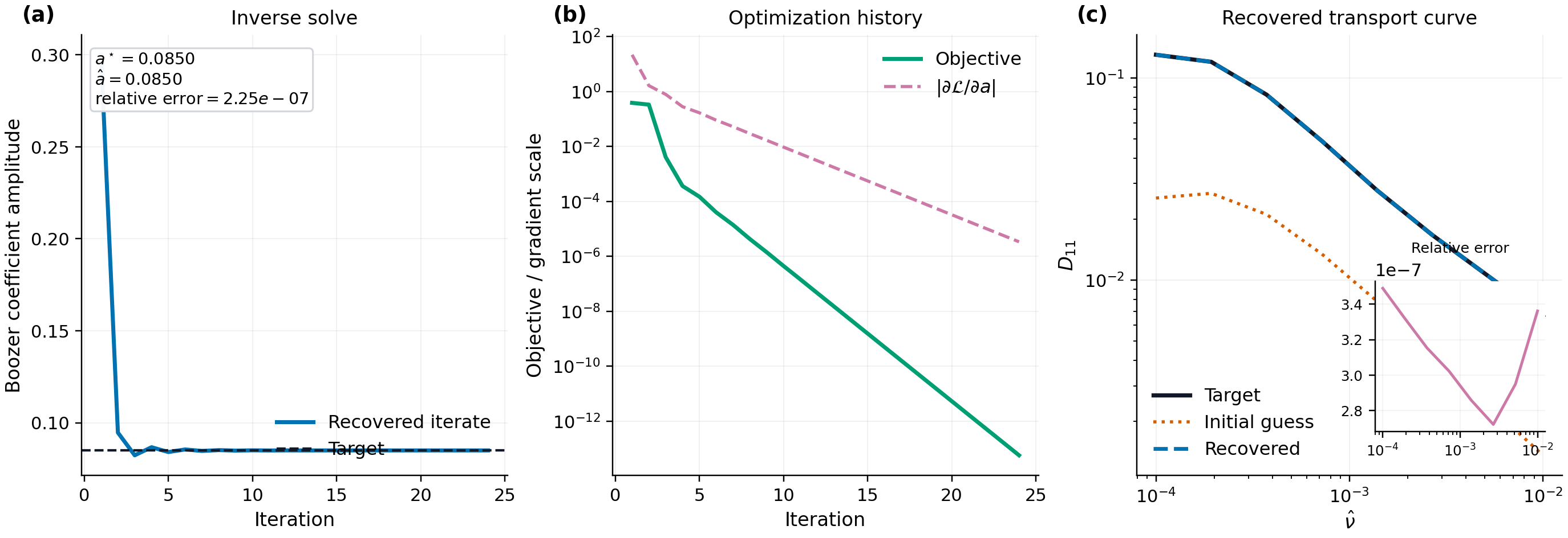
solves a small synthetic inverse problem on the analytic sample surface. One Fourier amplitude is treated as an unknown parameter, synthetic D11 observations are generated from a target surface, and JAX gradients are used to recover the amplitude.

The figure is written to:

docs/_static/autodiff_inverse_problem.png
docs/_static/autodiff_inverse_problem.pdf

It shows:

• parameter convergence

• objective reduction

• recovered transport response against the target response

Derivative Audit

The script:

python examples/derivative_audit.py

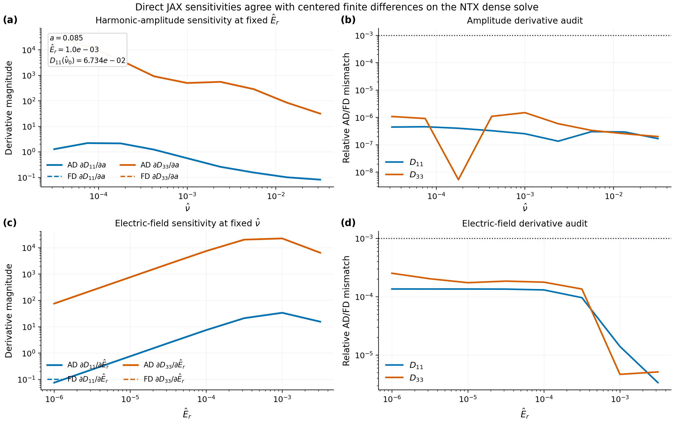
compares direct JAX gradients of the dense monoenergetic solve against centered finite differences for two practically important controls:

• a Boozer harmonic amplitude at fixed electric field,

• and the radial electric field at fixed collisionality.

The example does not rely on one hidden helper. It walks through the explicit prepared-solver workflow:

from ntx import (
    GridSpec,
    MonoenergeticCase,
    example_surface,
    prepare_monoenergetic_system,
    solve_prepared_coefficient_vector,
    solve_prepared_coefficient_vector_vjp,
)

That is the contract point for the prepared implicit-adjoint derivative path: the forward solve remains the same, while the backward rule stays isolated from user-facing optimization scripts.

The low-level operator derivative used by this path is now test-gated directly: tests/test_operators.py requires the hand-coded dD_k/dnu_hat and dD_k/depsi_hat blocks to match JAX differentiation of the assembled Legendre-space operator. This keeps the collisionality and radial-electric-field normalizations tied to the implemented equations rather than to a downstream finite-difference fit.

The figure is written to:

docs/_static/derivative_audit.png
docs/_static/derivative_audit.pdf

It shows:

• gradient magnitude across collisionality for D11 and D33,

• relative mismatch between autodiff and finite differences,

• electric-field sensitivities across \hat E_r,

• and the current numerical agreement used to validate the prepared implicit-adjoint path.

Prepared-Derivative Benchmark

The script:

python examples/derivative_path_benchmark.py

keeps the same prepared surface and the same D33 electric-field derivative, then times two user-visible paths:

• direct reverse-mode through solve_prepared_coefficient_vector(...),

• and the prepared custom-VJP path through solve_prepared_coefficient_vector_vjp(...).

The example is intentionally explicit. It shows how to:

• prepare a reusable system with prepare_monoenergetic_system(...),

• define scalar coefficient objectives,

• wrap them with jax.grad(...) and jax.vmap(...),

• JIT the resulting scan kernels,

• and compare timing and agreement on the same \hat E_r scan.

The figure is written to:

docs/_static/derivative_path_benchmark.png
docs/_static/derivative_path_benchmark.pdf

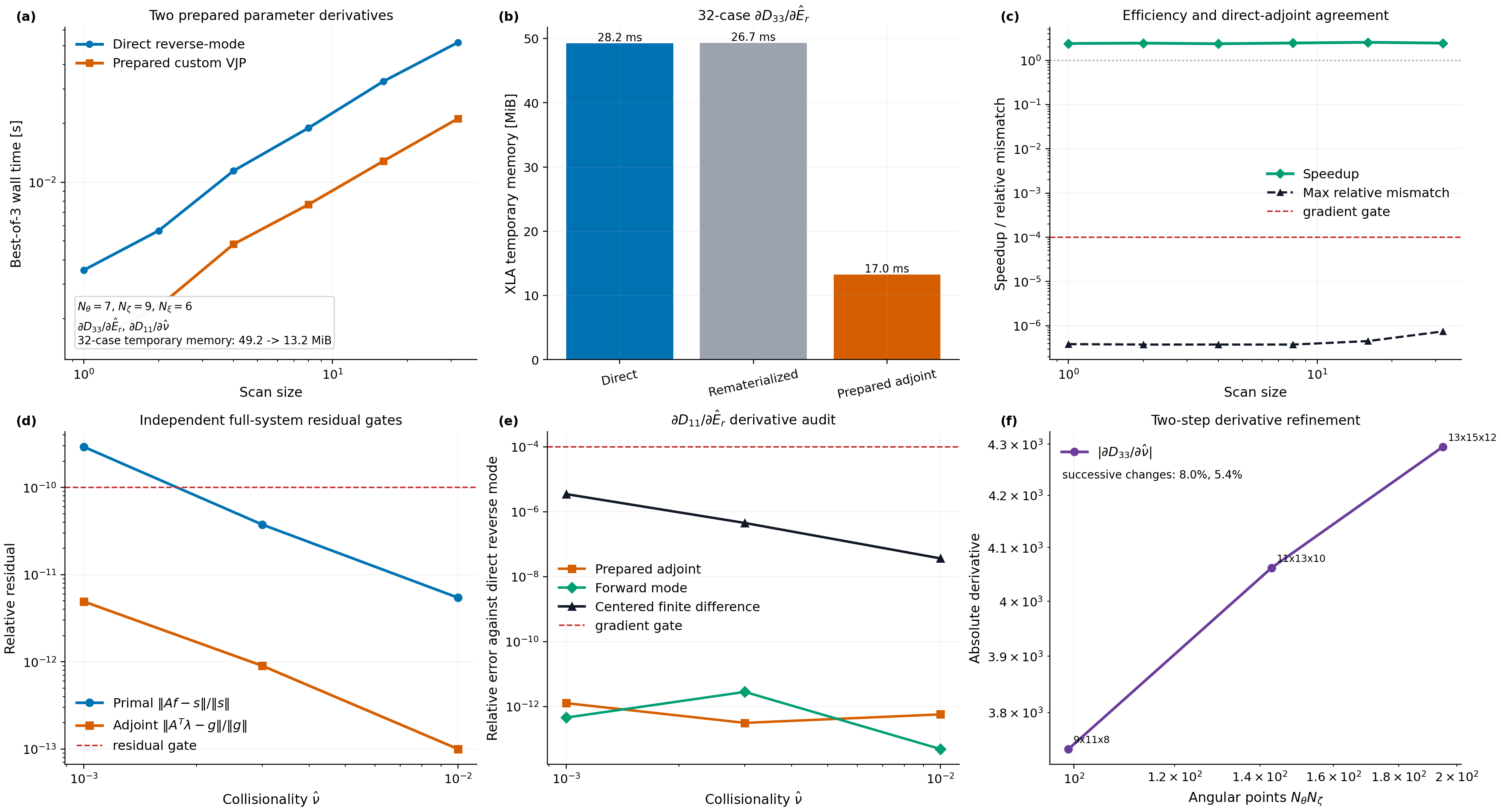
It shows:

• best-of-three wall times versus scan size,

• speedup of the prepared custom-VJP path,

• and the max relative mismatch between the two derivative paths.

The JSON sidecar is now checked by the physics-gate registry. The promoted release claim is derivative agreement, not benchmark-machine timing: the maximum prepared-vs-direct relative mismatch must remain below 1e-4; the reported speedup is retained as performance evidence.

Geometry-Control Derivative Benchmark

The script:

python examples/geometry_control_derivative_benchmark.py

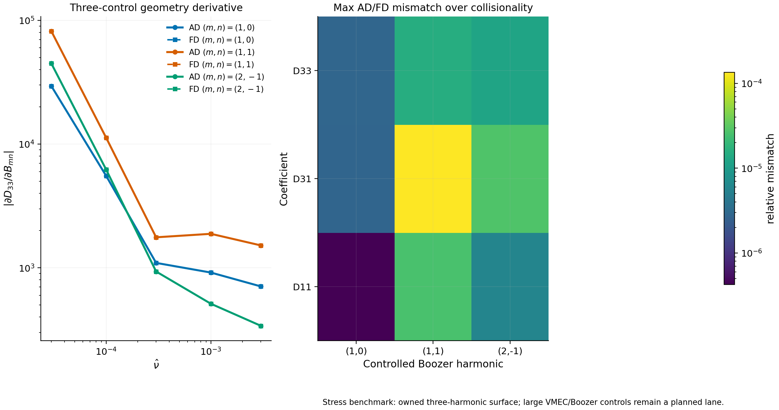
extends the derivative checks from one scalar control to three independent Boozer-harmonic amplitudes on the owned analytic surface. It compares direct JAX geometry-control derivatives against centered finite differences for D11, D31, and D33 across collisionality.

The figure is written to:

docs/_static/geometry_control_derivative_benchmark.png
docs/_static/geometry_control_derivative_benchmark.pdf
docs/_static/geometry_control_derivative_benchmark.json

This is an artifact-backed autodiff stress benchmark. It is not yet a large-geometry-control validation claim; the non-promoted follow-up is to transfer the same audit to reusable VMEC/Boozer geometry-control families and to compare geometry pullbacks with a prepared implicit-adjoint path once that pullback exists. The JSON sidecar is checked by the physics-gate registry with a current acceptance threshold of 2e-4 maximum relative direct-AD/finite-difference mismatch on this owned analytic surface.

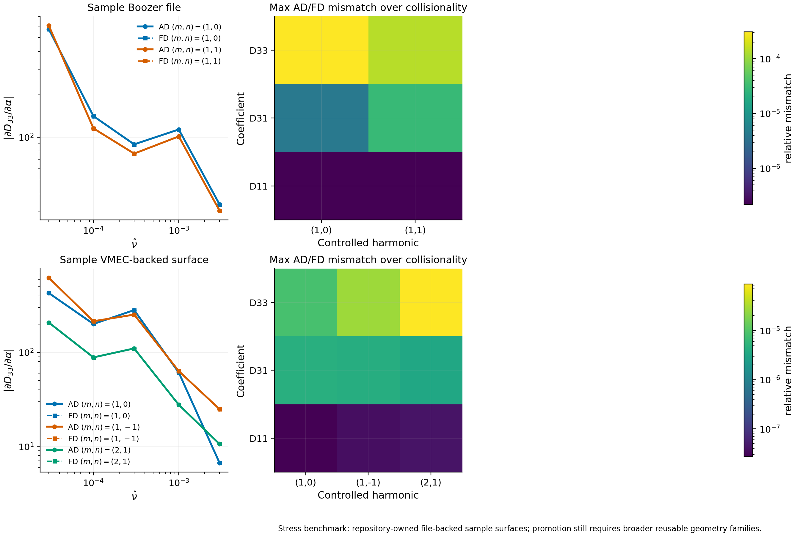
File-Backed Geometry-Control Benchmark

The script:

python examples/file_backed_geometry_control_derivative_benchmark.py

takes the next step on the geometry-control autodiff lane. Instead of the owned analytic surface, it loads two repository-owned file-backed cases:

• a Boozer-file sample surface,

• and a VMEC-backed sample surface.

For each case, NTX selects the dominant non-axisymmetric harmonics, perturbs them through dimensionless scale factors, and compares direct JAX derivatives against centered finite differences for D11, D31, and D33.

The figure is written to:

docs/_static/file_backed_geometry_control_derivative_benchmark.png
docs/_static/file_backed_geometry_control_derivative_benchmark.pdf
docs/_static/file_backed_geometry_control_derivative_benchmark.json

This closes the first file-backed slice of the geometry-control derivative path: the derivative audit now transfers from an owned analytic surface to repository-owned file-backed magnetic geometry. It is still a stress benchmark rather than a promoted design claim, since the non-promoted follow-up is a reusable family of VMEC/Boozer controls plus prepared implicit-adjoint geometry pullbacks. The committed JSON sidecar is now a physics gate with a 5e-4 maximum relative direct-AD/finite-difference mismatch threshold on the file-backed samples.

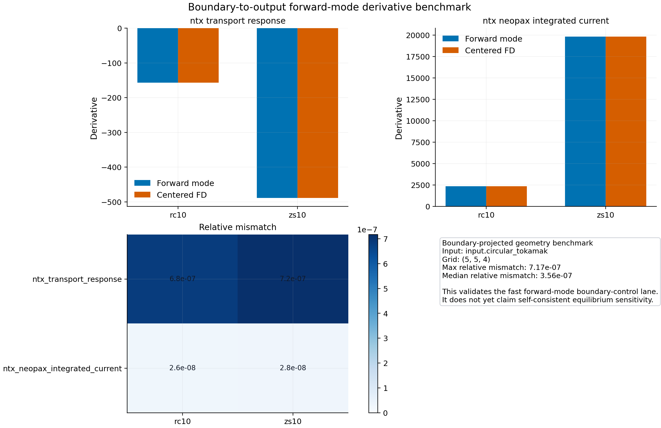
Boundary Forward-Mode Benchmark

The script:

python examples/boundary_forward_mode_current_derivative_benchmark.py

checks the next imported differentiable lane built on the upstream vmec_jax and booz_xform_jax packages. It treats two low-order boundary controls from the repository-owned sample input as independent variables, builds the boundary-projected VMEC state, transforms it to Boozer coordinates, and then differentiates two scalar outputs with respect to those controls:

• an NTX monoenergetic transport response,

• and an NTX+NEOPAX integrated-current objective.

The figure is written to:

docs/_static/boundary_forward_mode_current_derivative_benchmark.png
docs/_static/boundary_forward_mode_current_derivative_benchmark.pdf
docs/_static/boundary_forward_mode_current_derivative_benchmark.json

This is an artifact-backed stress benchmark for the boundary-to-output lane. It is intentionally scoped to the boundary-projected geometry map, where forward-mode autodiff matches centered finite differences on the committed sample case. It does not yet claim a fully validated self-consistent equilibrium sensitivity workflow for bootstrap current. The committed JSON sidecar is checked with a 1e-5 maximum relative forward-mode/finite-difference mismatch threshold.

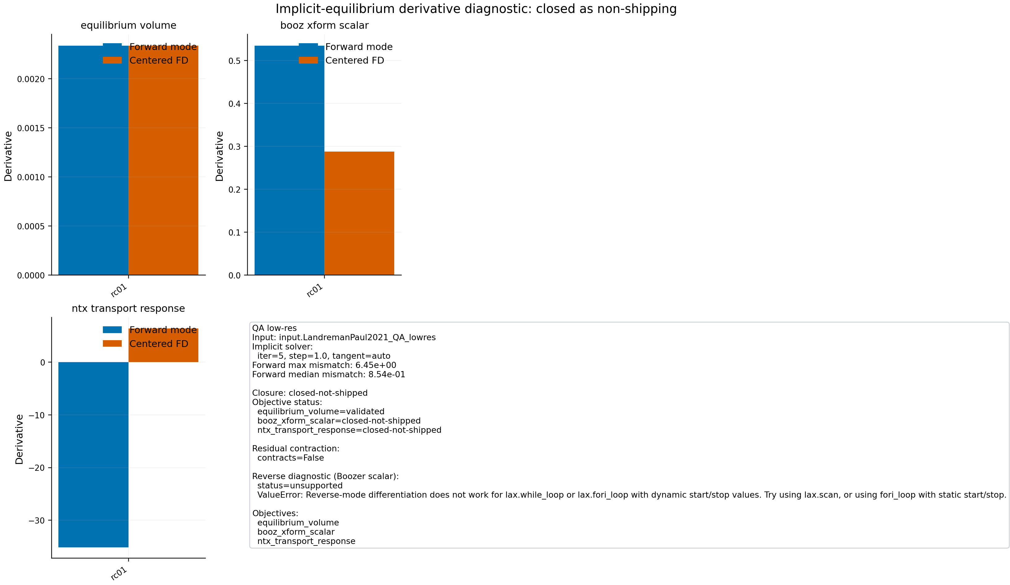
Implicit Equilibrium Forward-Mode Benchmark

The script:

python examples/implicit_equilibrium_forward_mode_derivative_benchmark.py

adds the next implicit-equilibrium diagnostic on the committed QA case. It uses the same low-order boundary controls, but now routes them through the implicit fixed-boundary vmec_jax residual solve with residual_tangent_mode="auto". The benchmark then differentiates three scalar outputs with respect to those controls:

• equilibrium volume,

• a Boozer-space scalar built from the implicit equilibrium,

• and an NTX monoenergetic transport response.

The figure is written to:

docs/_static/implicit_equilibrium_forward_mode_derivative_benchmark.png
docs/_static/implicit_equilibrium_forward_mode_derivative_benchmark.pdf
docs/_static/implicit_equilibrium_forward_mode_derivative_benchmark.json

This closes the implicit-equilibrium lane as a non-shipping diagnostic, not as a supported optimization path. The current JSON artifact shows a mixed result on the committed QA case:

• the equilibrium-volume derivative matches centered finite differences,

• the Boozer scalar fails tangent parity on the implicit lane,

• the NTX transport observable fails more strongly on the same lane,

• the residual history does not contract under the committed iteration ladder,

• and the matching reverse-mode Boozer-scalar diagnostic is unavailable because the dynamic-loop implicit solve is not a valid promoted reverse-mode path.

The JSON sidecar is intentionally registered as a monitored diagnostic, not an acceptance gate. The supported self-consistent equilibrium derivative route is the explicit-relaxed fixed-boundary lane below. The implicit lane should only be restored after the backend residual solve contracts and Boozer/NTX centered-FD tangent parity passes.

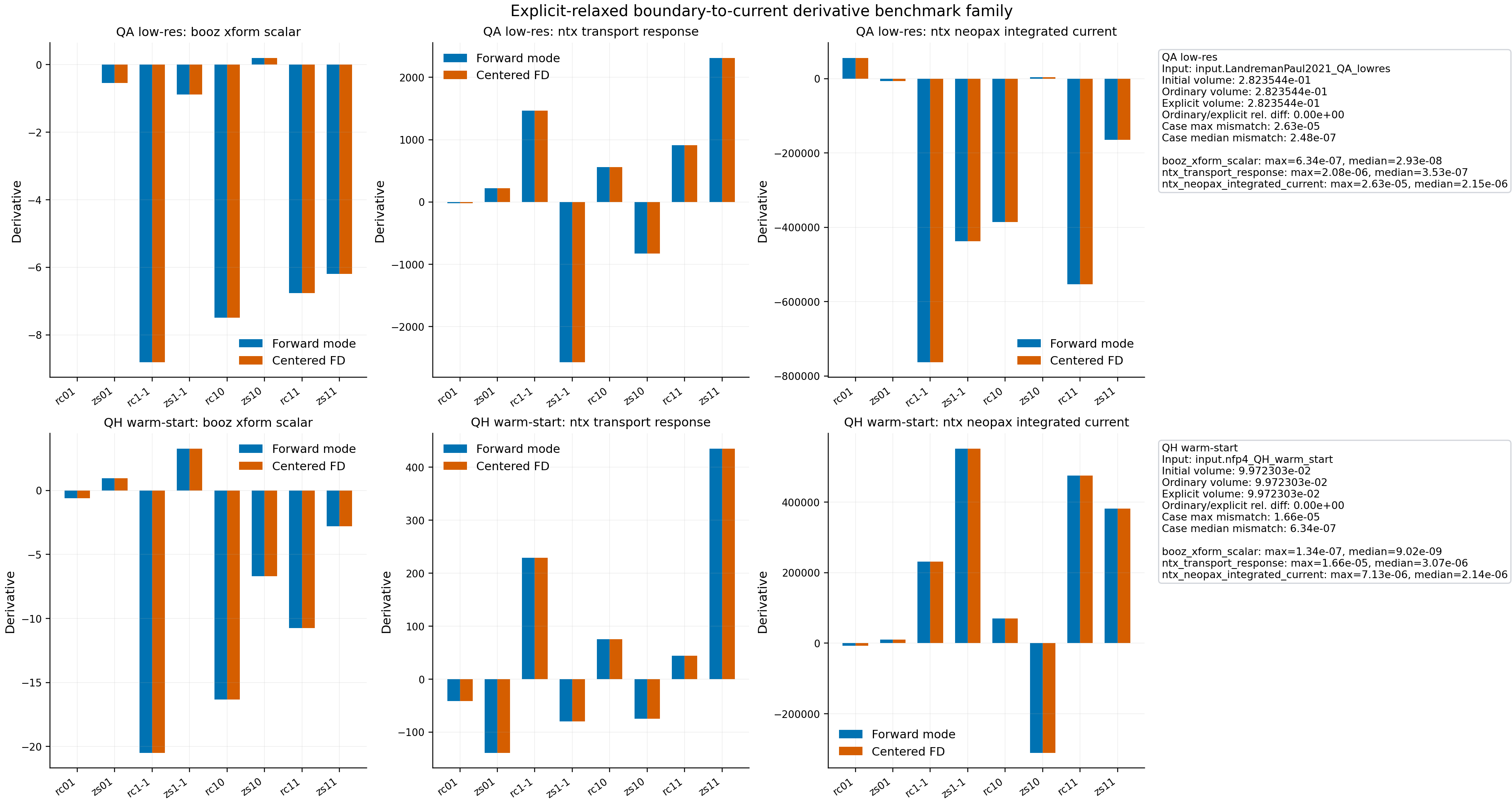
Explicit-Relaxed Equilibrium Benchmark

The script:

python examples/explicit_relaxed_boundary_current_derivative_benchmark.py

closes the next imported lane on two repository-owned non-axisymmetric cases: a low-resolution QA family input and a lighter QH warm-start input. It uses the same low-order boundary controls, but instead of stopping at the boundary-projected VMEC state it runs an explicitly relaxed fixed-boundary vmec_jax solve in a stable forward-mode regime and then differentiates three scalar outputs on each case:

• a Boozer-space scalar built from the relaxed surface,

• an NTX monoenergetic transport response,

• and an NTX+NEOPAX integrated-current objective.

The figure is written to:

docs/_static/explicit_relaxed_boundary_current_derivative_benchmark.png
docs/_static/explicit_relaxed_boundary_current_derivative_benchmark.pdf
docs/_static/explicit_relaxed_boundary_current_derivative_benchmark.json

This is the first committed self-consistent boundary-to-current forward-mode benchmark family. The JSON artifact records that the ordinary and explicit relaxed primal volumes agree on both committed cases, so the benchmark is not just an internally consistent autodiff loop on a different equilibrium branch. The non-promoted follow-up is now narrower:

• widen from the committed QA/QH cases to additional geometry families,

• add integrated-current objectives on the supported explicit-relaxed lane,

• and repair reverse mode on the relaxed-equilibrium lane.

The committed JSON sidecar is now checked by the physics-gate registry with a 1e-4 maximum relative forward-mode/finite-difference mismatch threshold. The artifact also reports the ordinary-vs-explicit-relaxed volume difference, which is currently zero on the committed cases.

At the moment, the reverse-mode implicit diagnostic remains non-shipping for a concrete reason: the matching QA Boozer-scalar probe is unavailable or guarded to zero while centered finite differences are nonzero, so it is not a promoted sensitivity workflow.

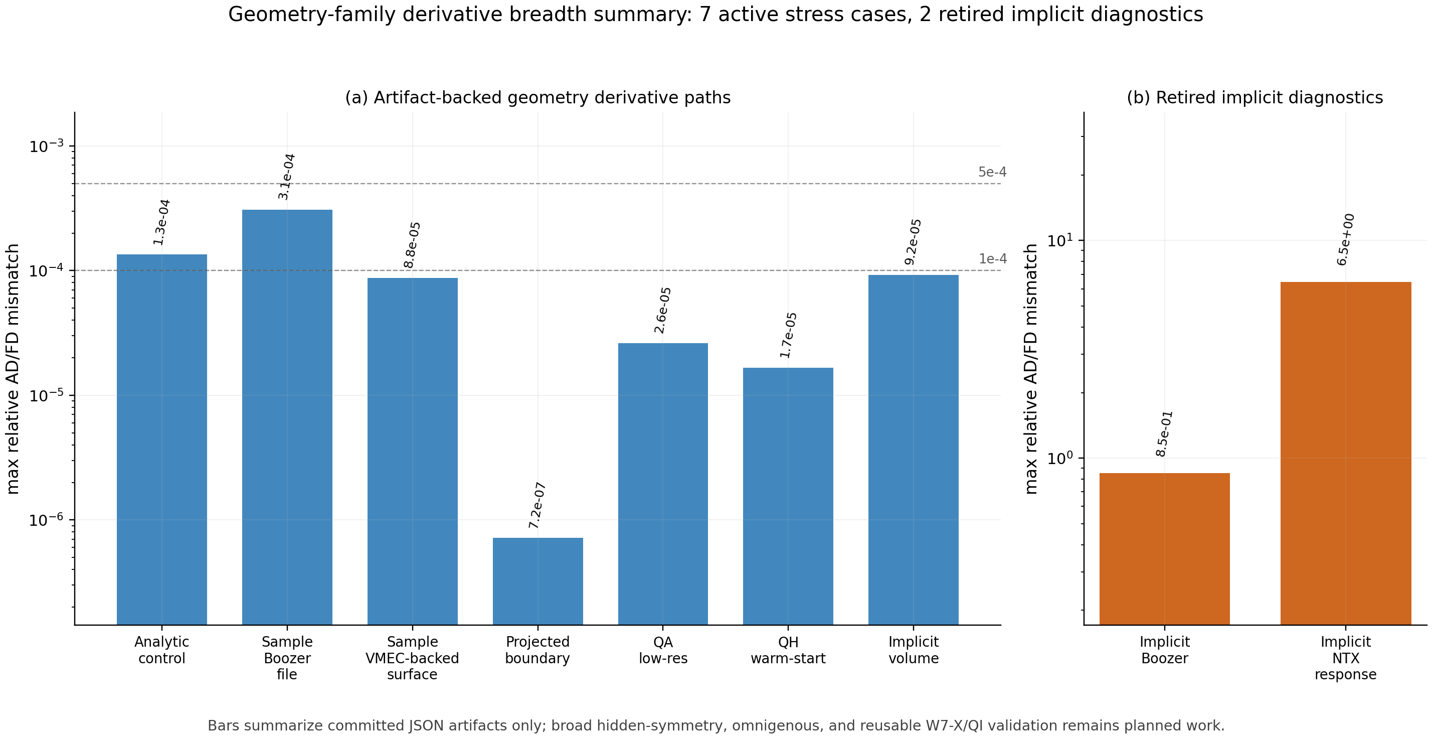
Geometry-Family Breadth Summary

The script:

python examples/geometry_family_breadth_summary.py

does not rerun expensive equilibrium solves. It reads the committed derivative artifacts and summarizes the current geometry-breadth status in one publication-ready figure:

• analytic geometry-control derivatives,

• file-backed Boozer and VMEC geometry-control derivatives,

• boundary-projected current derivatives,

• explicit-relaxed QA/QH boundary-to-current derivatives,

• and the implicit-equilibrium diagnostic split into the validated volume objective and the retired non-shipping Boozer/NTX transport diagnostics.

The figure is written to:

docs/_static/geometry_family_breadth_summary.png
docs/_static/geometry_family_breadth_summary.pdf
docs/_static/geometry_family_breadth_summary.json

This closes the artifact-backed geometry-breadth summary lane, not the full geometry-family validation lane. The remaining promotion requirements are explicit in the JSON sidecar: broader W7-X/QI/omnigenous inputs, direct D11/D31/D33 parity and convergence ladders, and implicit Boozer/transport derivative parity.

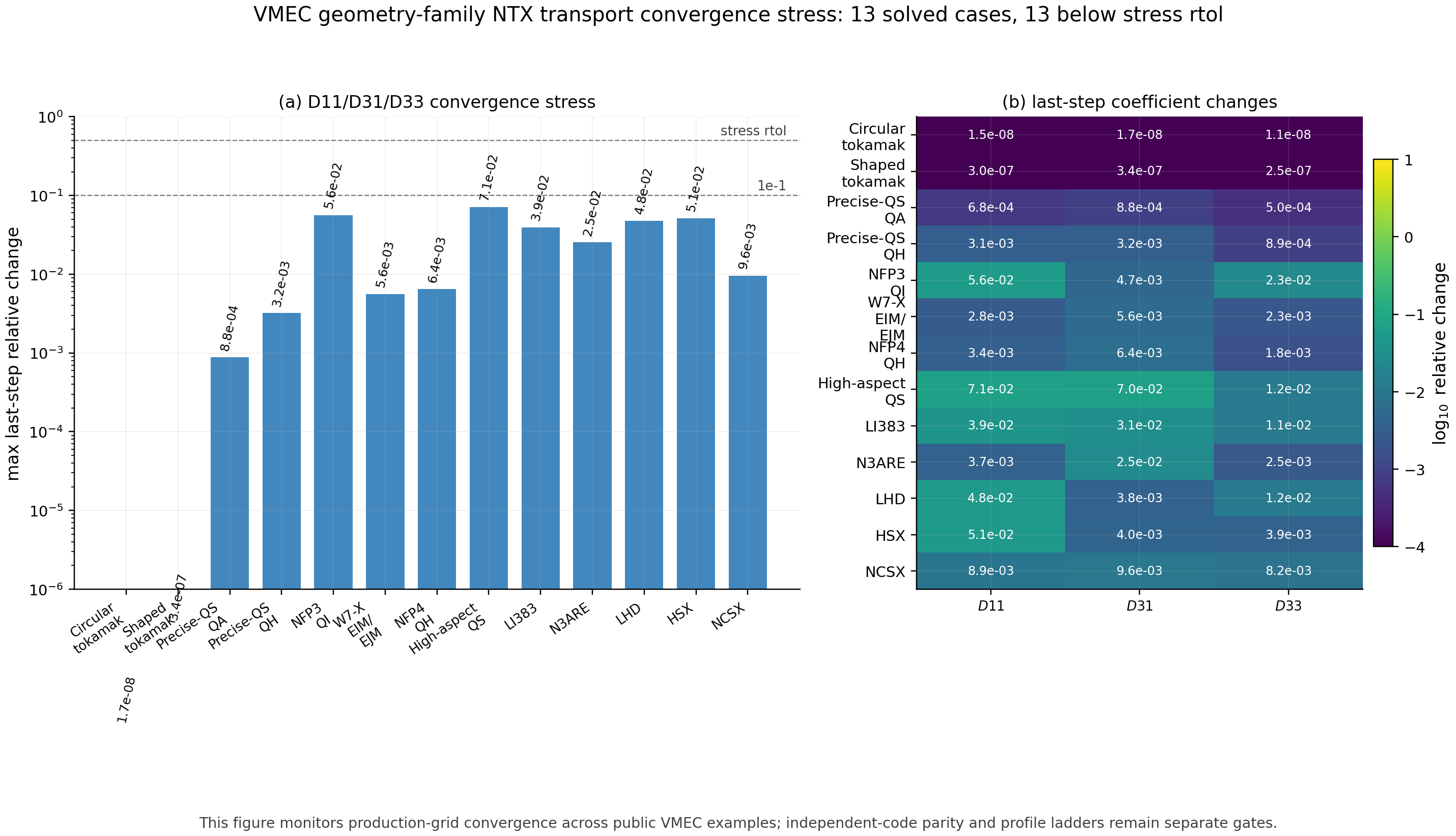
Geometry-Family Transport Convergence

The script:

python examples/geometry_family_transport_convergence.py --preset production

discovers reusable VMEC wout examples from local vmec_jax, STELLOPT, and SIMSOPT checkouts, loads each surface through the NTX VMEC path, and runs a production D11/D31/D33 grid ladder. The JSON also stores D13 and the normalized Onsager residual so coefficient convergence and reciprocity quality are audited together. The figure and JSON sidecar are written to:

docs/_static/geometry_family_transport_convergence.png
docs/_static/geometry_family_transport_convergence.pdf
docs/_static/geometry_family_transport_convergence.json

The current artifact is a convergence stress diagnostic across the available public geometry families. It distinguishes cases that are below the tracked stress tolerance from cases that need profile-ladder or independent-reference promotion work.

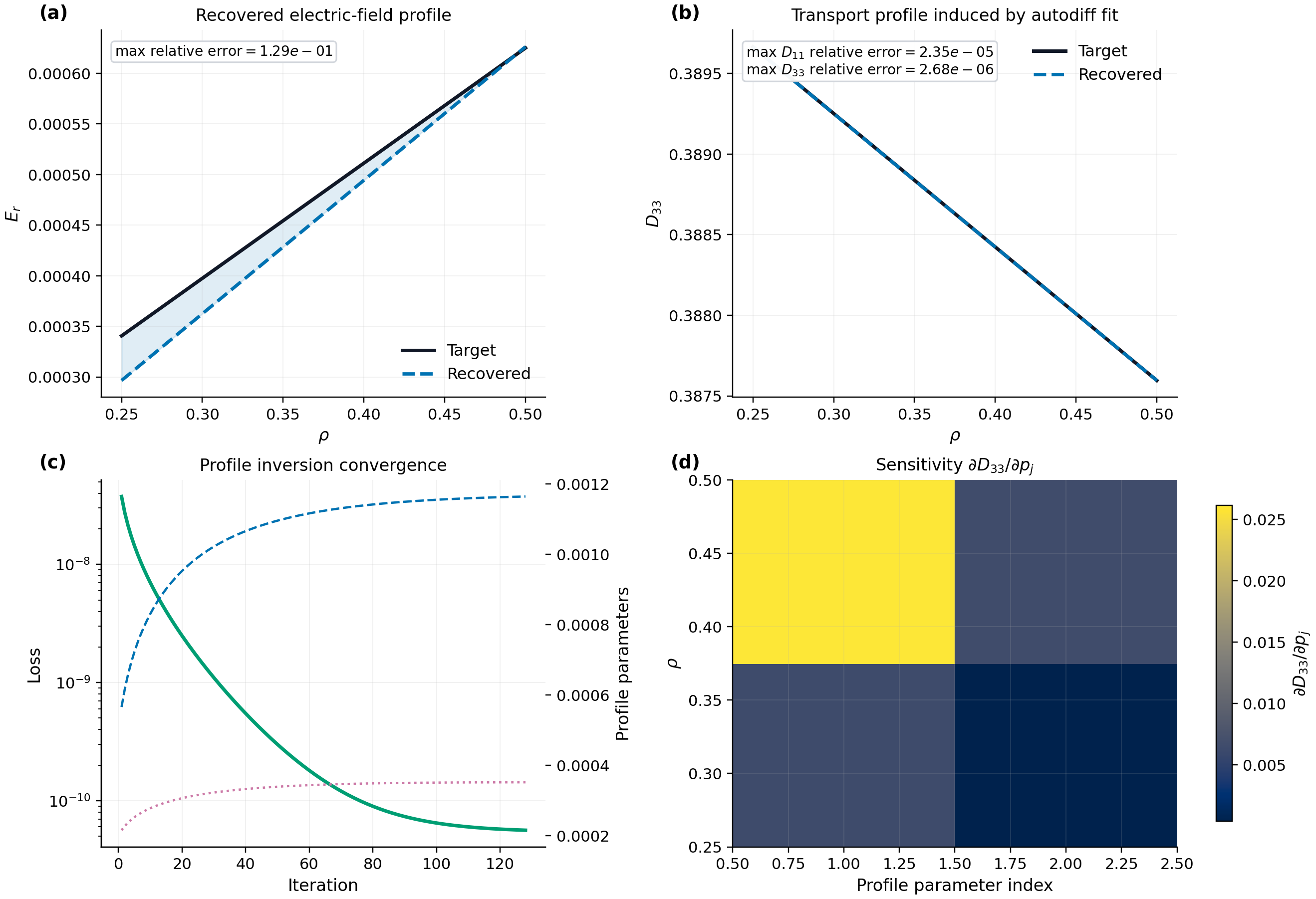
NEOPAX-Style Profile Example

The script:

python examples/neopax_autodiff_profiles.py

builds a small NTX scan, maps it into the NEOPAX monoenergetic data layout, and then solves a low-dimensional electric-field profile inversion using autodiff.

The figure is written to:

docs/_static/autodiff_neopax_profiles.png
docs/_static/autodiff_neopax_profiles.pdf

It shows:

• target and recovered radial electric-field profiles

• target and recovered D33 profiles

• objective reduction

• the local sensitivity of D33 to the profile parameters

The fast test suite now gates this interpolation layer directly: tests/test_autodiff.py checks that D33 sensitivities through the electric-field profile basis agree with centered finite differences on a controlled coefficient table. This keeps the profile inverse-design and uncertainty examples tied to a checked differentiable map instead of relying only on end-to-end objective reduction.

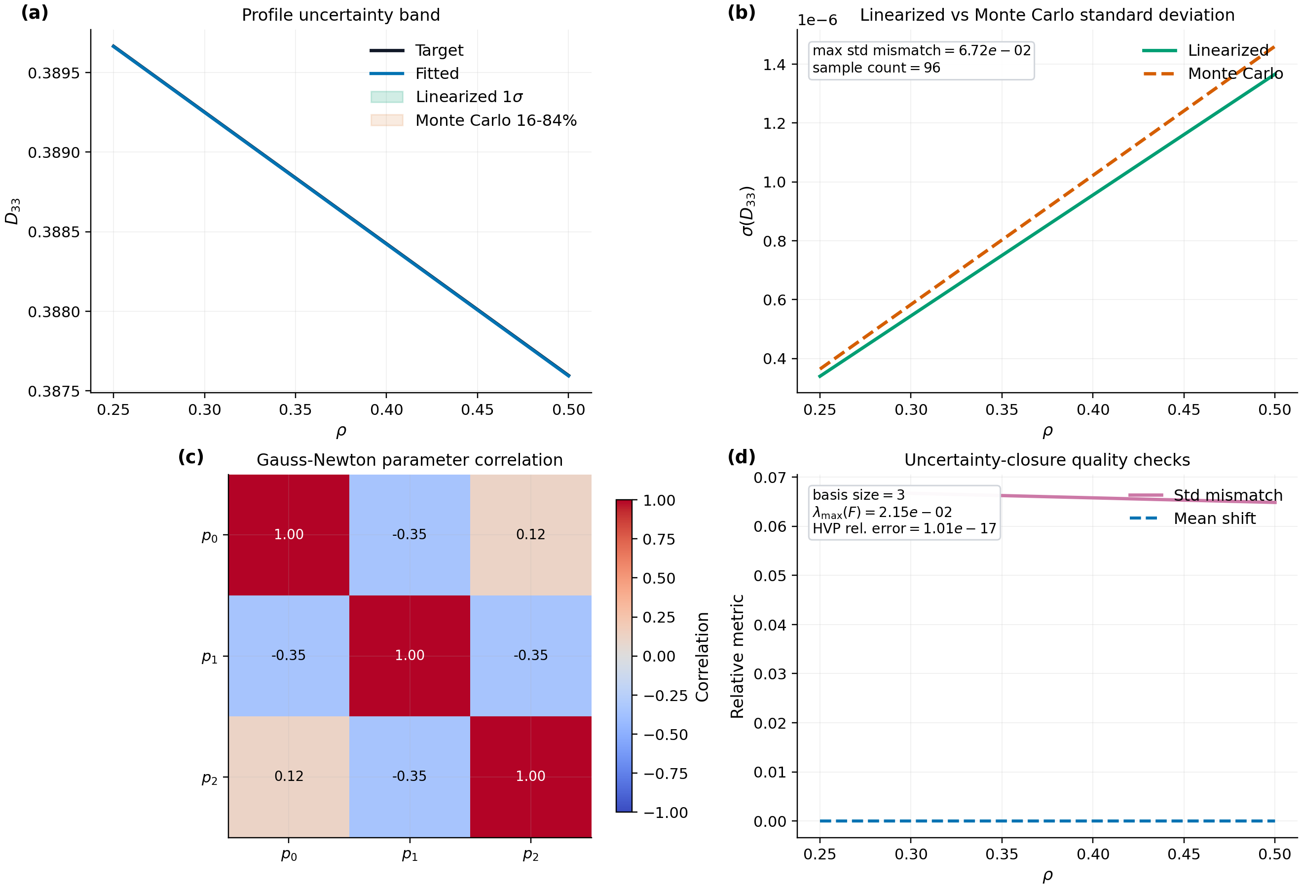
Profile Uncertainty Audit

The script:

python examples/autodiff_profile_uncertainty.py

uses the same differentiable NEOPAX-style profile fit, then compares two uncertainty-propagation paths for the recovered D33(\rho) profile under a small prescribed Gaussian uncertainty on the fitted radial electric-field basis parameters:

• a linearized covariance propagation through the sensitivity matrix,

• and a small Monte Carlo ensemble in the fitted profile-parameter space.

The committed artifact uses a three-term odd-power radial basis by default and also records a local Fisher/Gauss-Newton matrix plus a Hessian-vector-product probe for the same combined D11/D33 residual used by the fit. The HVP probe is evaluated at the recovered profile parameters, where the residual term vanishes, so it should agree with the Fisher/Gauss-Newton product. This provides a local mathematical gate for profile-UQ derivatives without promoting the synthetic profile family to a broad design claim.

The figure is written to:

docs/_static/autodiff_profile_uncertainty.png
docs/_static/autodiff_profile_uncertainty.pdf
docs/_static/autodiff_profile_uncertainty.json

It shows:

• the fitted transport profile with propagated uncertainty bands,

• linearized versus Monte Carlo standard deviations,

• the fitted profile-parameter correlation matrix,

• the relative mismatch between the two uncertainty paths,

• and the Fisher/HVP consistency metrics stored in the JSON artifact.

This is the current artifact-backed uncertainty-propagation benchmark for the autodiff lane. It is intentionally synthetic and is tracked as a monitored stress benchmark rather than a parity gate, but it exercises the same differentiable profile map used in inverse-design and profile-control studies.

Robust Bootstrap-Current Optimization

The script:

python examples/bootstrap_current_robust_optimization.py

adds a prescribed Gaussian uncertainty on the scalar geometry control used by the bootstrap-current response optimization and compares:

• the deterministic objective landscape,

• the robust mean-minus-risk objective,

• the optimized nominal current profile,

• and the uncertainty band of that profile under the prescribed control perturbation.

The figure is written to:

docs/_static/bootstrap_current_robust_optimization.png
docs/_static/bootstrap_current_robust_optimization.pdf
docs/_static/bootstrap_current_robust_optimization.json

This is a synthetic robust-design benchmark anchored to the same differentiable current-response workflow as the main optimization example. It is currently a tracked stress diagnostic, not a literature-grade validation claim. The JSON artifact separates robust_objective_relative_change, which gates the optimization workflow, from weighted_current_ratio, which is a signed current-profile diagnostic and should not be interpreted as a standalone parity claim.

Parallel Execution

Large scans do not need to stay on one device. NTX currently exposes two parallel paths:

from ntx import solve_monoenergetic_parallel_scan
from ntx import solve_monoenergetic_multiprocess_scan

solve_monoenergetic_parallel_scan(...) keeps execution inside one Python process and is the lightest-weight option when all visible devices are healthy. solve_monoenergetic_multiprocess_scan(...) runs one worker process per device and is the robust option when the platform shows process-local solver behavior.

For local profiling:

python scripts/profile_parallel_runtime.py --output-json parallel-runtime.json
python scripts/profile_multiprocess_runtime.py --backend cpu --workers 2

For multi-CPU emulation on a workstation, start the script in a fresh process with:

XLA_FLAGS=--xla_force_host_platform_device_count=4 python scripts/profile_parallel_runtime.py

On the office workstation, the single-process path exposes a cuSolver failure mode on cuda:1, while the multiprocess pinned-device path is numerically correct on both GPUs. For the repository smoke cases the multiprocess path is still slower than the serial batched solve because worker startup dominates, so it should be treated as a throughput lane for larger scans rather than a default for small studies.