Performance

NTX now includes explicit scaling benchmarks and figure-generation helpers for serial batched scans and the multiprocess throughput lane. It also now includes workflow profilers for the archive-backed fixed-field closure audit and the corrected integrated W7-X workflow.

Reusable Prepared Scans

Repeated scans on one geometry should use a prepared fixed-shape solver:

import jax.numpy as jnp
from ntx import (
    GridSpec,
    compile_prepared_scan_solver,
    example_surface,
    prepare_monoenergetic_system,
)

prepared = prepare_monoenergetic_system(example_surface(), GridSpec(17, 25, 16))
scan = compile_prepared_scan_solver(prepared)
report = scan.warmup()
coefficients = scan(jnp.logspace(-5, -2, 128))

The object pads only the final chunk and reuses one batch shape across scan lengths. Supported fixed buckets are 1, 8, 32, and 128. Automatic mode uses sequential lax.map with bucket 8 on CPU and GPU. Explicit execution_mode and batch_size arguments exist for measured crossover studies, not as claims that wider vectorization is always faster or equally accurate.

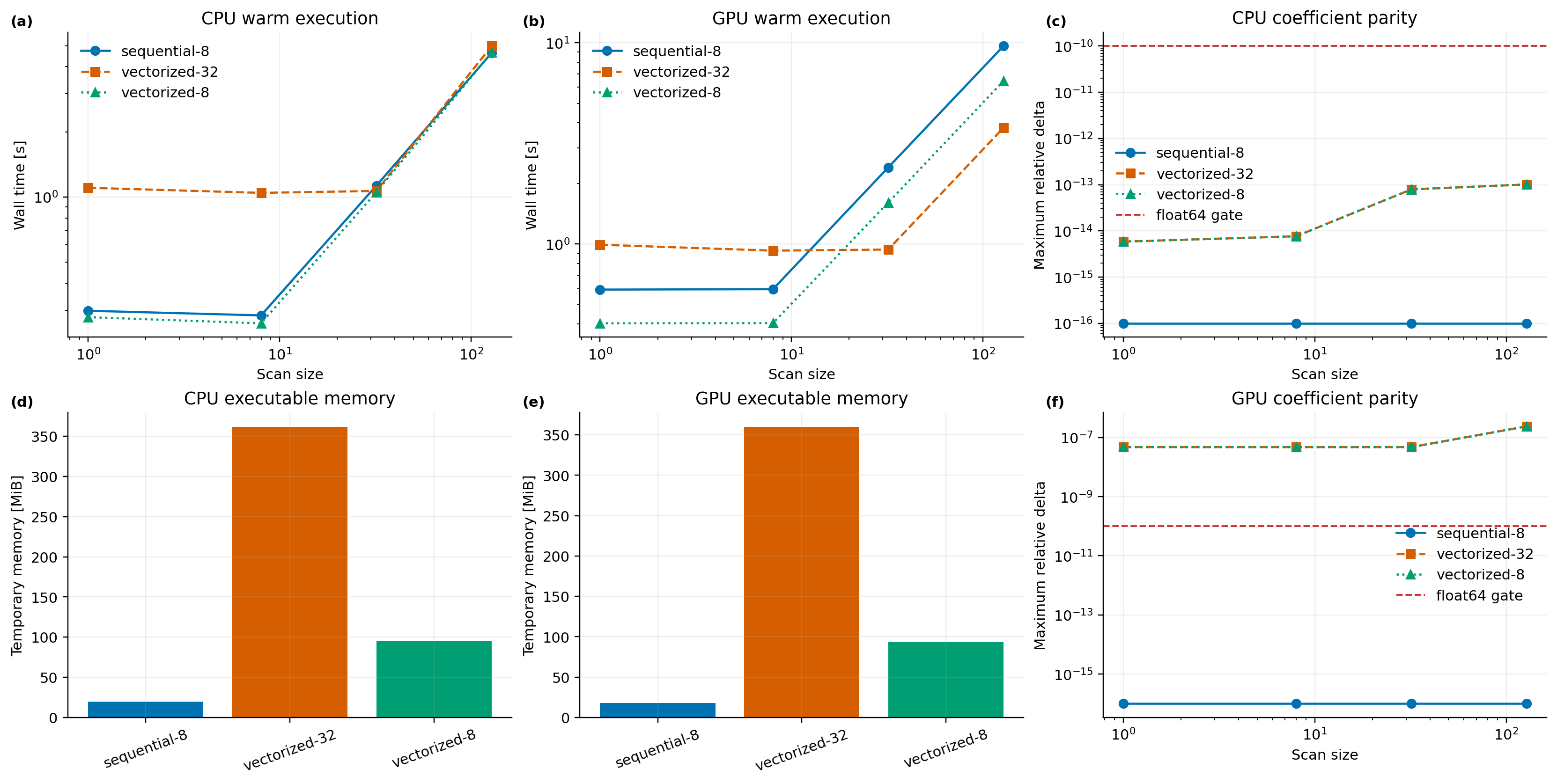
warmup() reports lowering, compilation, first execution, warm execution, argument/output size, and executable temporary memory separately. The production CPU audit on the bundled DKES surface at 17 x 25 x 16 found about 20.7 MiB of executable temporary memory for sequential width 8, compared with 100.3 MiB for vectorized width 8 and 379.1 MiB for vectorized width 32. The wider modes were only modestly faster and were not uniformly faster over scan sizes 1, 8, 32, and 128, so bounded sequential execution remains the CPU default. Coefficients agreed within 2.6e-11 absolute in that map; float64 acceptance remains 1e-10 relative/absolute with appropriate near-zero scaling.

Buffer donation was evaluated for both fixed-batch input arrays on the same production grid. XLA reported both buffers as unusable for donation and kept temporary memory unchanged at 20,656,504 bytes. NTX therefore does not invalidate user-owned collisionality or electric-field arrays for a nonexistent memory benefit.

On the office RTX A4000 with JAX 0.6.2, vectorized width 32 is about 2.5x faster than sequential width 8 at 128 cases, but differs from the canonical compiled scalar solve by up to 2.4e-7 relative over the production scan. The sequential scan is bitwise identical to that compiled scalar reference. Since the vectorized path fails the 1e-10 float64 parity gate, it remains explicit and non-default pending a stable batched-factorization/refinement result.

Larger-grid GPU results keep the same conclusion:

Grid	Mode	Temporary memory	Warm fixed-batch execution	Maximum relative delta
`17 x 25 x 16`	sequential-8	`18.0 MiB`	`0.594 s`	`0` vs compiled scalar
`17 x 25 x 16`	vectorized-8	`94.1 MiB`	`0.404 s`	`2.4e-7` over scan
`25 x 31 x 24`	sequential-8	`55.1 MiB`	`3.48 s`	`0` vs sequential reference
`25 x 31 x 24`	vectorized-8	`280.2 MiB`	`3.00 s`	`2.4e-8`
`25 x 25 x 63`	sequential-8	`36.9 MiB`	`10.23 s`	`0` vs sequential reference
`25 x 25 x 63`	vectorized-8	`182.4 MiB`	`9.78 s`	`3.1e-7`
`25 x 25 x 140`	sequential-8	`36.9 MiB`	`10.98 s`	reference mode

The Nxi=140 first execution was 66.5 s despite a 1.06 s reported XLA compile stage, while subsequent execution was about 11 s. This likely includes backend initialization/autotuning and is why the benchmark does not fold first execution into either compile or warm solve time. Both office GPUs reproduced the production-grid runtime and vectorized discrepancy. The owned JSON files are prepared_scan_gpu_25x31x24.json, prepared_scan_gpu_25x25x63.json, and prepared_scan_gpu_25x25x140.json under docs/_static.

If JAX returns a resource-exhaustion exception, the prepared solver adds guidance to select sequential execution and bucket 1 or 8. A hard driver or process termination cannot be intercepted in Python; production users should start from the documented sequential memory map before increasing vector width.

The cache is optional and should be configured before compilation:

from ntx import configure_compilation_cache

configure_compilation_cache(
    "~/.cache/ntx/jax",
    minimum_compile_seconds=1.0,
    explain_cache_misses=False,
)

Generate synchronized crossover artifacts with:

python scripts/benchmark_prepared_scan.py \
  --backend cpu --surface dkes --sizes 1,8,32,128 \
  --n-theta 17 --n-zeta 25 --n-xi 16 \
  --output-json docs/_static/prepared_scan_cpu_production.json

python examples/prepared_scan_performance.py \
  --cpu-json docs/_static/prepared_scan_cpu_production.json \
  --gpu-json docs/_static/prepared_scan_gpu_production.json \
  --output-prefix docs/_static/prepared_scan_performance

Prepared scan CPU/GPU runtime, memory, and parity

Both old scaling harnesses now call jax.block_until_ready inside the timed region. This is required for valid asynchronous accelerator measurements.

File-Backed Run Path

The TOML/CLI path prepares the geometry and derivative operators once, then reuses that prepared system for the solve and output writer. This avoids the old double geometry evaluation in file-backed single-case runs and lowers both runtime and peak transient array pressure. Verbose CLI runs print separate prepare, solve, write, plot, and total timings.

NetCDF and HDF5 outputs are written uncompressed for fast inspection and cross-code exchange. Use .npz when smaller Python-only artifacts matter more than write speed:

ntx input.toml --output outputs/run.nc --plot
ntx input.toml --output outputs/run.npz

Benchmark Scripts

Collect scaling data:

python scripts/benchmark_scaling.py --backend cpu --surface dkes --sizes 8,16,32,64
python scripts/benchmark_scaling.py --backend gpu --surface dkes --sizes 16,32,64 --workers 2
python scripts/benchmark_strong_scaling.py --backend cpu --surface dkes --num-cases 64
python scripts/benchmark_prepared_scan.py --backend cpu --surface dkes --sizes 1,8,32,128

Generate publication-style figures:

python examples/performance_scaling.py \
  --cpu-json docs/_static/performance_scaling_cpu_smoke.json \
  --gpu-json docs/_static/performance_scaling_gpu_smoke.json \
  --figure-title "Smoke-grid serial vs multiprocess scaling" \
  --output-prefix docs/_static/performance_scaling_smoke

python examples/performance_strong_scaling.py \
  --cpu-json docs/_static/performance_strong_scaling_cpu_production.json \
  --gpu-json docs/_static/performance_strong_scaling_gpu_production.json \
  --figure-title "Production fixed-workload strong scaling" \
  --output-prefix docs/_static/performance_strong_scaling_production

The example writes PNG, PDF, and JSON summary outputs. The summary JSON records CPU/GPU crossover cases, process peak resident memory, device counts, and serial-vs-parallel coefficient deltas.

For the committed production-grid map:

XLA_FLAGS=--xla_force_host_platform_device_count=4 \
python scripts/benchmark_scaling.py \
  --backend cpu --surface dkes --sizes 16,32,64,128 \
  --workers 4 --n-theta 17 --n-zeta 25 --n-xi 16 \
  --output-json docs/_static/performance_scaling_cpu_production.json

python examples/performance_scaling.py \
  --cpu-json docs/_static/performance_scaling_cpu_production.json \
  --gpu-json docs/_static/performance_scaling_gpu_production.json \
  --figure-title "Production-grid serial vs parallel scaling" \
  --output-prefix docs/_static/performance_scaling_production

XLA_FLAGS=--xla_force_host_platform_device_count=4 \
python scripts/benchmark_strong_scaling.py \
  --backend cpu --surface dkes --num-cases 128 \
  --worker-counts 1,2,4 --device-counts 1,2,4 \
  --n-theta 17 --n-zeta 25 --n-xi 16 \
  --output-json docs/_static/performance_strong_scaling_cpu_production.json

Profile the corrected integrated W7-X workflow:

python scripts/profile_w7x_integrated_workflow.py \
  --output-json examples/outputs/profile_w7x_integrated_workflow/profile.json \
  --cprofile-out examples/outputs/profile_w7x_integrated_workflow/profile.pstats \
  --trace-dir examples/outputs/profile_w7x_integrated_workflow/trace

The script records:

cached scan/database timings
first-call and steady-state closure timings
resident memory
a Python cProfile dump
a TensorFlow/JAX trace that can be opened in TensorBoard or Perfetto

Smoke-Grid Scaling

Figure assets:

docs/_static/performance_scaling_smoke.png
docs/_static/performance_scaling_smoke.pdf
docs/_static/performance_scaling_smoke.json

Smoke-grid scaling

Interpretation:

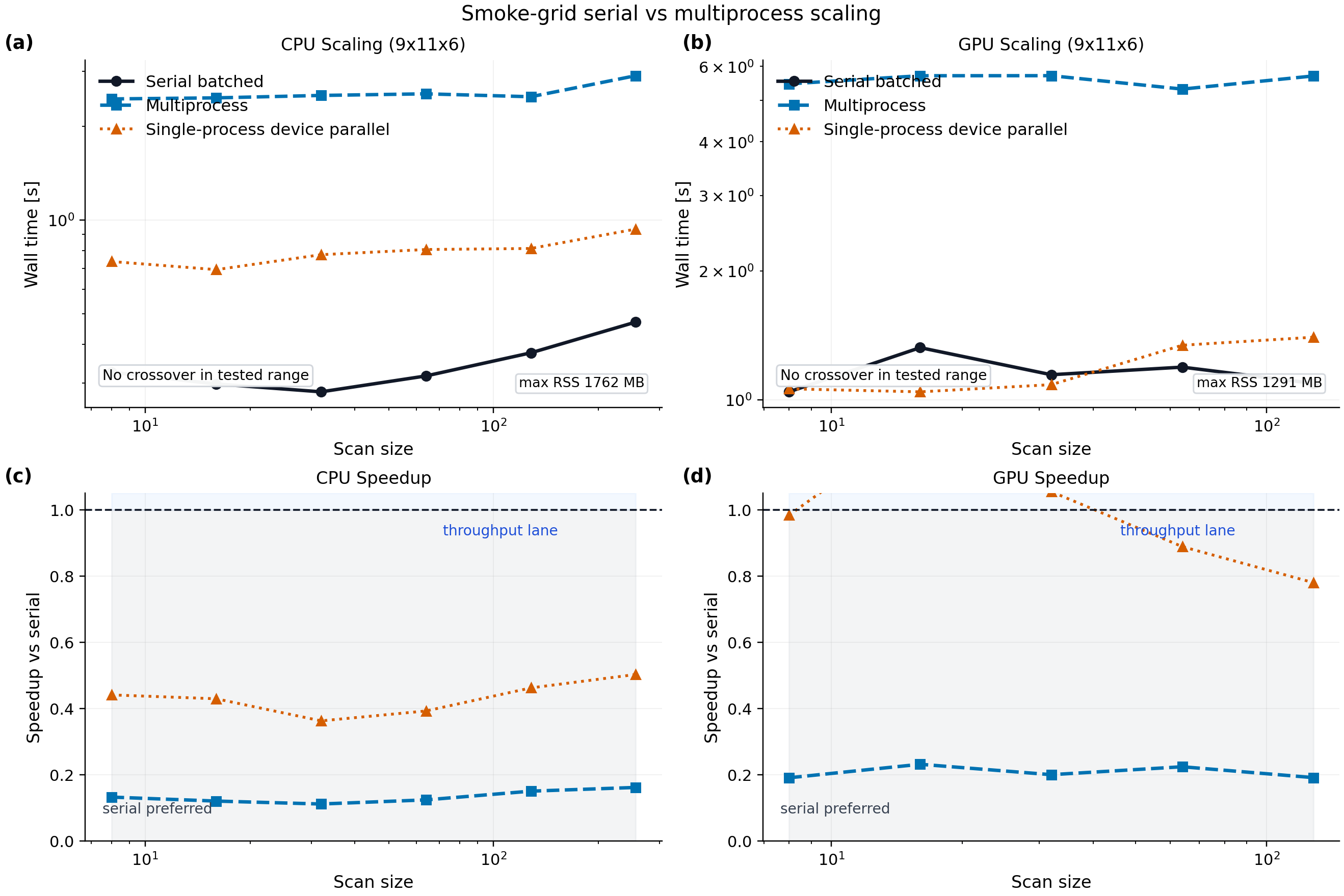
on the repository smoke grid 9 x 11 x 6, serial batched JAX is the default choice on both CPU and GPU for small and medium scans
the smallest GPU point is startup dominated and should not be interpreted as a real throughput crossover
on the refreshed local CPU run, the multiprocess and single-process device-parallel lanes are numerically correct but still slower than serial over the tested smoke-grid range
the refreshed CPU smoke artifact reports process peak resident memory of about 1.76 GB
the refreshed office GPU smoke artifact reports process peak resident memory of about 1.29 GB, with one of two GPUs passing the single-process device-parallel smoke filter

Heavier-Grid Scaling

Figure assets:

docs/_static/performance_scaling_heavy.png
docs/_static/performance_scaling_heavy.pdf
docs/_static/performance_scaling_heavy.json

Heavier-grid scaling

Interpretation:

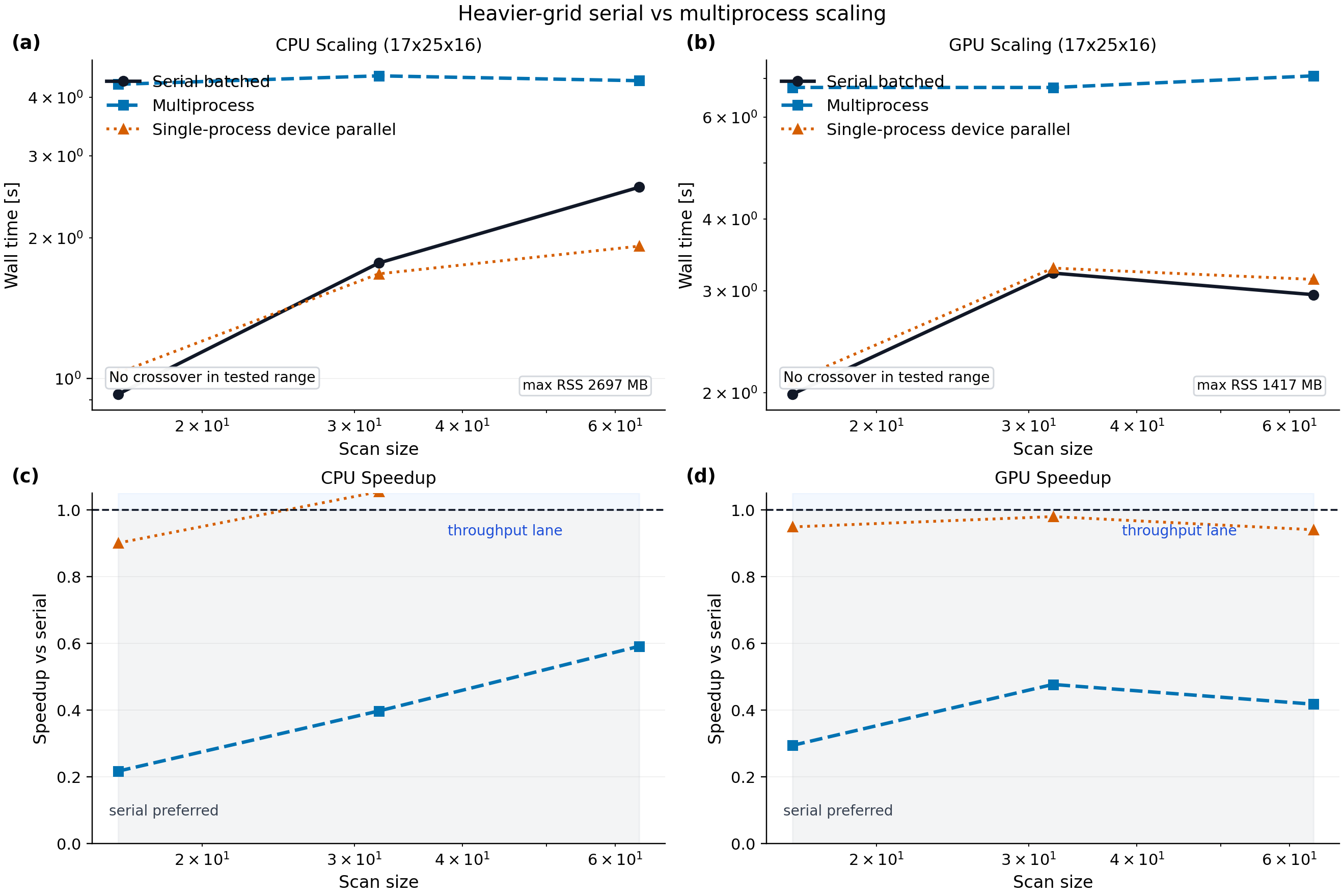
on the heavier DKES grid 17 x 25 x 16, the refreshed local CPU artifact shows the single-process device-parallel lane crossing serial by 32 cases, while the 4-worker CPU multiprocess lane remains slower through 64 cases
on the same heavier grid, the office 2-GPU multiprocess lane remains slower than serial in the tested range under the current shared-office software and hardware stack
the refreshed CPU heavy artifact reports process peak resident memory of about 2.70 GB
the refreshed office GPU heavy artifact reports process peak resident memory of about 1.42 GB, again with one healthy single-process device
the practical guidance from these measurements is:
- use serial batched JAX for small and medium studies
- use the single-process device-parallel lane on CPU only after checking that the target grid/scan size has crossed over
- use the multiprocess lane only when a measured workload shows enough amortization of process startup on the target machine
- treat office multi-GPU multiprocess execution as a robust isolation path first, and as a throughput path only after benchmarking the specific production workload

Production-Grid Scaling

Figure assets:

docs/_static/performance_scaling_production.png
docs/_static/performance_scaling_production.pdf
docs/_static/performance_scaling_production.json

Production-grid scaling

Interpretation:

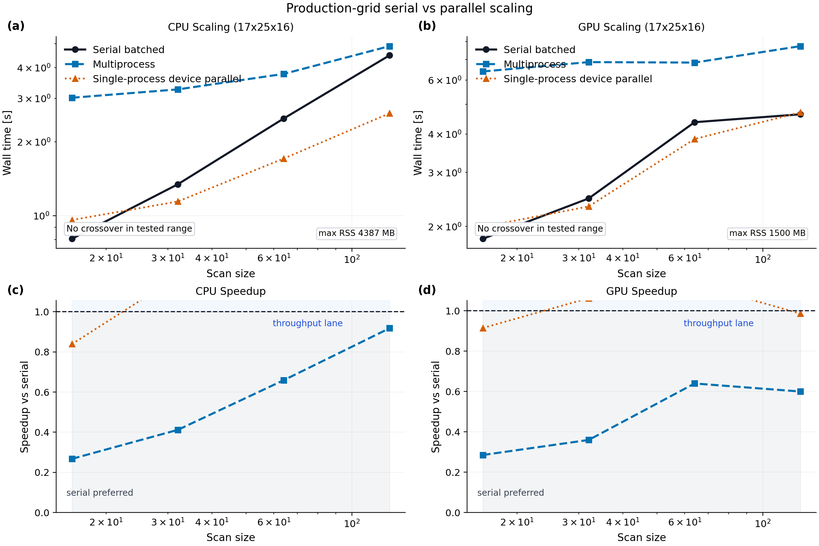
the committed production map uses the same 17 x 25 x 16 DKES-style grid as the heavier-grid artifact but extends the scan ladder to 128 cases
with four logical CPU devices exposed to JAX, the single-process device-parallel lane crosses serial at 32 cases and reaches a best observed speedup of about 1.72x at 128 cases
the 4-worker CPU multiprocess lane remains below serial through 128 cases, reaching about 0.92x; process startup and duplicated runtime state still dominate this workload
the office two-GPU workstation run found two CUDA devices, but only one device passed the NTX smoke solve for single-process parallel execution under the tested software stack
on that GPU workload, single-process device-parallel timing is characterized and numerically identical to serial for D11, but multiprocess remains below serial through 128 cases
peak resident memory is about 4.39 GB for the 4-device CPU run and 1.50 GB for the tested GPU run

The production-grid guidance is therefore:

use compiled prepared-geometry reuse first when the geometry and array shapes are fixed
use single-process JAX device parallelism for CPU scan ladders after a local crossover measurement
keep multiprocess and multi-GPU execution as workload-specific isolation or throughput paths until the exact target grid shows a measured win

Production Strong Scaling

Figure assets:

docs/_static/performance_strong_scaling_production.png
docs/_static/performance_strong_scaling_production.pdf
docs/_static/performance_strong_scaling_production.json

Production strong scaling

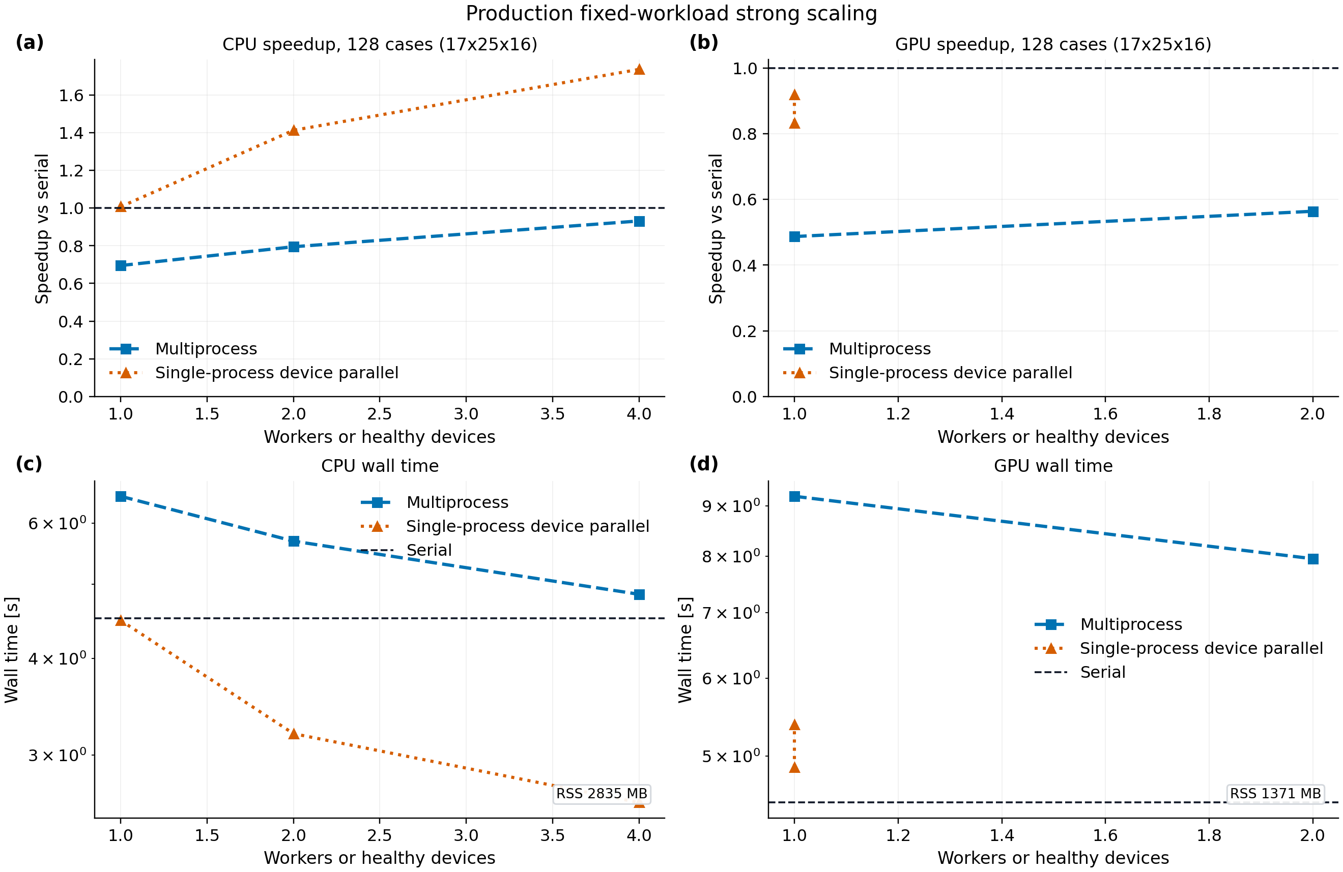
Interpretation:

the committed strong-scaling map fixes the workload at 128 cases on the 17 x 25 x 16 DKES-style grid, then varies workers or requested devices
on CPU, single-process device parallelism scales from 1.01x at one exposed device to 1.74x at four devices; the corresponding efficiency drops from startup parity to about 0.43 at four devices, so this is useful but not ideal strong scaling
on CPU, the multiprocess lane improves with more workers but remains below serial at 0.93x for four workers, which confirms that process startup and duplicated runtime state are still too costly for this fixed workload
on the tested two-GPU workstation, both CUDA devices are visible but only one passes the NTX single-process smoke solve; the strong-scaling artifact therefore records one healthy parallel GPU and does not promote multi-GPU speedup
all CPU and GPU strong-scaling lanes reproduce serial D11 to the committed numerical tolerance; the largest GPU multiprocess delta is about 2.34e-8
peak resident memory is about 2.83 GB for the CPU strong-scaling run and 1.37 GB for the GPU strong-scaling run

This closes the first artifact-backed strong-scaling lane. The next performance work should target device-health reproducibility and larger VMEC-family workloads before claiming general multi-GPU scaling.

Prepared-Geometry Reuse

The prepared-geometry reuse artifact isolates the repeated fixed-geometry solve path from the multiprocess throughput lane:

python examples/prepared_geometry_reuse_profile.py --preset paper

For targeted trace capture:

python examples/prepared_geometry_reuse_profile.py \
  --preset smoke --case-counts 3 \
  --trace-dir examples/outputs/ntx_prepared_geometry_profile/cpu_smoke_trace \
  --perfetto \
  --device-memory-profile examples/outputs/ntx_prepared_geometry_profile/cpu_smoke_trace/device_memory.prof

Figure assets:

docs/_static/prepared_geometry_reuse_profile.png
docs/_static/prepared_geometry_reuse_profile.pdf
docs/_static/prepared_geometry_reuse_profile.json

Prepared-geometry reuse

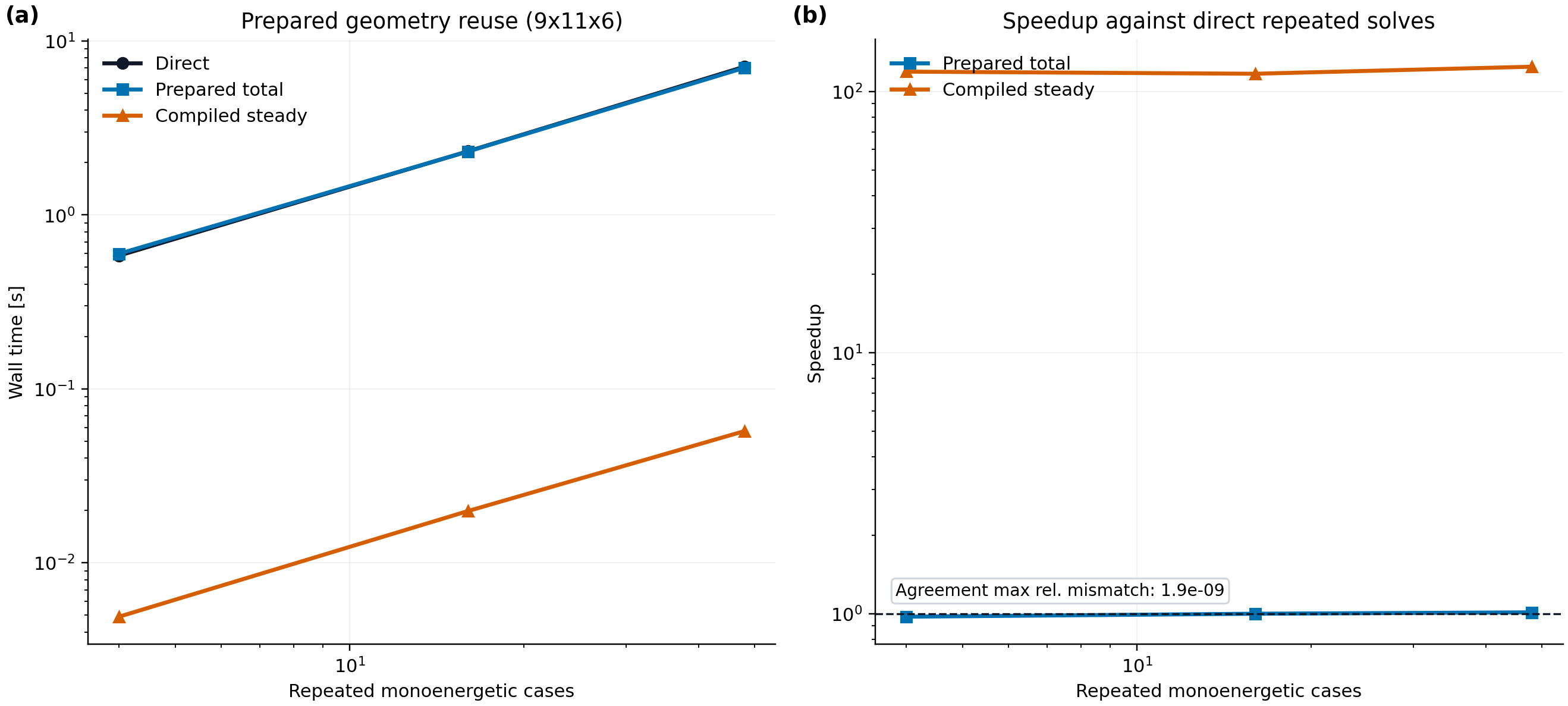
Current local CPU interpretation:

direct repeated solves and un-jitted prepared solves are near parity after one warmup solve, so hoisting geometry arrays alone is not the main win on this grid
the compiled prepared steady path reaches a best observed speedup of about 1.50e2x against direct repeated solves with maximum coefficient mismatch below 2e-9
the first compiled call is still visible at about 0.43 s, which confirms that optimization workflows should compile once per fixed geometry and reuse stable shapes across collisionality, electric-field, species, and radial axes
the process peak resident memory in this run is about 1.24 GB

This turns the speed lane into a concrete engineering target: stabilize and reuse prepared compiled closures before deeper linear-algebra rewrites or multi-process orchestration.

Finite-Beta RHSMode=1 Profile-Current Profiling

The finite-beta profile-current lane now has a dedicated handoff note for the same-contract SFINCS-JAX RHSMode=1 bottleneck:

docs/sfincs-jax-rhsmode1-profile-current-handoff.md

The current profiling result is:

SFINCS-JAX 1.1.0 at df0c70d completes the 13 x 15 x 8, Nx=5 three-radius smoke profile-current artifact in 24.7 s total on local CPU; all three HDF5 outputs pass the true-residual metadata gate
the same checkout completes the 17 x 21 x 12, Nx=5 inner-radius HDF5 output in 9.90 s wall time with 1.55 GB max RSS, sparse_pc_gmres, and true-residual/target 8.45e-7
a three-radius 25 x 31 x 17, Nx=11 production ladder completes in 383.16 s with about 9.46 GB max RSS and true-residual gates passing at every radius
the pitch-resolution audit shows the remaining RHSMode=1 profile-current discrepancy is not a residual failure: the accepted high-Nxi even/odd Legendre stress gap is 1.323e-1, below the current 1.5e-1 reduced-closure tolerance
a same-grid collisionOperator=0 full-collision probe timed out after 901.76 s and about 9.97 GB max RSS without a completed current output

The old sparse-solver runtime lane and the reduced-closure pitch stress lane are closed under the documented tolerances. The full-collision branch remains a non-shipping feasibility diagnostic rather than a release blocker.

QI Hires NEOPAX-Database Export

The downstream QI finite-beta hires database-generation command exercises the largest public examples/build_neopax_scan_from_ertilde.py path used so far: 25 x 25 x 60, seven radial surfaces, and the default 16 x 12 (nu_v, Er_tilde) scan per surface. The current script reports per-surface timing and accepts --scan-batch-size to split that flattened scan into fixed-size chunks.

Measured on the local CPU for one radial surface with the same QI hires VMEC/Boozer files:

full-surface batching: 64.7 s, about 5.0 GB peak RSS
--scan-batch-size 32: 55.9 s, about 1.46 GB peak RSS
--scan-batch-size 16: 75.3 s, about 1.27 GB peak RSS
XLA_FLAGS=--xla_force_host_platform_device_count=4 with --parallel-devices 4 --scan-batch-size 32: 47.7 s for the same one-surface workload on the local CPU, with coefficient differences from the serial batched run at roundoff

For CPU runs of that example, start with --scan-batch-size 32. For GPU runs, leave full-surface batching enabled when memory permits; add a batch size only when the device runs out of memory at higher resolution.

--scan-batch-size primarily reduces peak memory; it is not a CPU parallelism switch. For CPU-only laptops that are still too slow, expose multiple JAX host devices before launch and request per-surface scan sharding:

XLA_FLAGS=--xla_force_host_platform_device_count=4 \
python examples/build_neopax_scan_from_ertilde.py \
  --wout examples/inputs/wout_QI_nfp2_newNT_opt_hires.nc \
  --booz examples/inputs/boozermn_wout_QI_nfp2_newNT_opt_hires.nc \
  --surface-backend vmec \
  --device-backend cpu \
  --parallel-devices 4 \
  --scan-batch-size 32 \
  --output examples/input/Dij_NTX.h5

The script reports the resolved batch size, requested parallel device count, and visible backend. If the collaborator command still includes --device-backend gpu on a CPU-only machine, it will fail before solving; use --device-backend cpu or omit the flag on laptops without a configured JAX GPU.

Reproducibility

The figure JSON payloads committed in docs/_static/ are:

performance_scaling_cpu_smoke.json
performance_scaling_gpu_smoke.json
performance_scaling_cpu_heavy.json
performance_scaling_gpu_heavy.json
performance_scaling_cpu_production.json
performance_scaling_gpu_production.json
performance_scaling_production.json
performance_strong_scaling_cpu_production.json
performance_strong_scaling_gpu_production.json
performance_strong_scaling_production.json
prepared_geometry_reuse_profile.json

Fresh runs of scripts/benchmark_scaling.py and scripts/profile_parallel_runtime.py also record process peak resident memory as max_rss_mb. That value is intentionally treated as a run-environment metric rather than a parity target, but it keeps memory visible whenever timing artifacts are regenerated. The committed CPU artifacts were refreshed locally; the committed GPU artifacts were refreshed from a clean temporary checkout on the office GPU workstation. For CI smoke coverage, scripts/profile_parallel_runtime.py accepts --num-cases and --grid so the serial/device-parallel correctness path can run on a tiny grid while the default command remains the profiling workload.

They were collected on:

local workstation CPU with XLA_FLAGS=--xla_force_host_platform_device_count=4
office workstation GPU with XLA_PYTHON_CLIENT_PREALLOCATE=false

Integrated W7-X Workflow

The corrected integrated W7-X raw branch is now the right profiling target because the database normalization is closed there and the rebuilt workflow matches the shipped reference current tightly.

Current local CPU profile, using the cached rebuilt W7-X scan:

reference_load_seconds: 1.04e-2
scan_prepare_seconds: 2.94e-4
rebuilt_scan_load_seconds: 2.69e-3
field_species_seconds: 1.97
database_seconds: 2.55e-1
no_momentum_first_seconds: 8.64
no_momentum_steady_seconds: 2.63e-2
momentum_correction_first_seconds: 8.81
momentum_correction_steady_seconds: 1.58e-2
current_reduction_seconds: 3.29e-2
max_rss_mb: about 1847

Interpretation:

the corrected integrated workflow is compile-bound on first call, not arithmetic-bound
the steady-state closure path is already fast on CPU once compiled
the main performance priority is therefore to reduce recompiles and tracing, not to micro-optimize the final current reduction

The current cProfile dump is dominated by XLA compilation:

about 15 s in backend_compile_and_load
about 20 s total Python runtime

That points directly to the next speed lane:

stabilize shapes and dtypes in the closure path
hoist and reuse the compiled no-momentum and momentum-correction calls
avoid retracing/vmap rebuilding across repeated workflow invocations
then revisit deeper kernel/vectorization work only after those compile overheads are under control

A simple persistent compilation-cache experiment is now also bounded out as a first-order fix. Re-running the same workflow in a fresh process with --compilation-cache-dir enabled leaves the first-call latencies essentially unchanged:

cold cached process:
- no_momentum_first_seconds: 1.17e+1
- momentum_correction_first_seconds: 1.24e+1
warm cached process:
- no_momentum_first_seconds: 1.17e+1
- momentum_correction_first_seconds: 1.23e+1

So the current integrated workflow is not being held back by a missing on-disk compilation cache alone. The speed lane should stay focused on shape stability, static-argument control, and reusable compiled closure calls rather than on cache toggles by themselves.

SOLVAX Solver Migration

The generated block-solver migration was measured against the immediately preceding NTX implementation on the same prepared 13 x 15 x 32 analytic solve, with 21 warm samples and identical float64 coefficients:

Device	Metric	Before	SOLVAX
Apple CPU	warm median	20.54 ms	20.30 ms
Apple CPU	executable temporary memory	4.91 MB	4.02 MB
Apple CPU	compile	0.297 s	0.362 s
RTX A4000	warm median	51.02 ms	47.43 ms
RTX A4000	executable temporary memory	4.57 MB	3.99 MB
RTX A4000	compile	0.938 s	1.123 s

The migration improves warm CPU/GPU runtime and reduces temporary memory by about 18% on CPU and 13% on GPU. Cold compilation is about 20–22% slower, so this is not presented as an across-the-board speedup. Prepared executable reuse remains necessary for production scans. A separate pre/post coefficient ladder at N_xi = 2, 16, 32, 63, 140 agrees to approximately 1e-13 or better.

Research-Grade Performance Plan

The next performance work should stay evidence-driven:

measure compile time, first-call time, steady-state time, peak resident memory, and device memory separately;
keep small PR tests and large profiling campaigns separate;
profile the exact workload before changing linear algebra, vectorization, or dependencies;
prefer stable shapes and prepared data structures over dynamic Python control inside jit;
promote multi-process or multi-device paths only when a measured production grid crosses over from serial batched JAX.

JAX-specific rules for NTX:

use jax.vmap for independent collisionality, electric-field, species, or radial scan axes when all mapped leaves have compatible shapes;
use jax.lax.scan for fixed-length iterative loops that would otherwise be unrolled inside jit;
keep static arguments hashable, immutable, and low-cardinality so they do not create unnecessary recompiles;
consider buffer donation only at public call boundaries where the caller will not reuse the donated arrays;
use jax.profiler.trace or XProf/Perfetto for targeted traces, and JAX memory profiling for OOM or retained-buffer investigations;
for GPU sharing, set explicit memory policy such as XLA_PYTHON_CLIENT_PREALLOCATE=false or XLA_PYTHON_CLIENT_MEM_FRACTION before launching concurrent runs.

SOLVAX and Equinox are useful but not automatic wins:

SOLVAX owns generic generated block elimination, reusable factors, transpose solves, and algebraic residuals; NTX retains the physics operator and source assembly. Further abstraction is accepted only with measured runtime or memory benefit.
Equinox should be evaluated for typed PyTree modules and filtered transforms only if it simplifies static-versus-dynamic argument handling or custom derivative APIs without destabilizing the public NTX API.

Do not use broad XLA dump passes as the default profiling loop on normal workstations. They are useful for focused compiler investigations, but the current project bottlenecks are better attacked with smaller traces, shape audits, and cached closure-only profiling.